flac2mp3 – Batch FLAC to MP3 Converter

When you have a massive music library in lossless FLAC format and need portable MP3 copies, doing it manually is not an option. flac2mp3 is a clean Python script that recursively finds all FLAC files and converts them to high-quality MP3 using ffmpeg.

Why flac2mp3?

The script uses libmp3lame encoder with -q:a 0 — the highest Variable Bit Rate quality setting. The audible difference from the original FLAC is virtually nonexistent, while file sizes drop dramatically.

Features

  • Recursive search: Walks through all subdirectories, finds every .flac file automatically.
  • Multiple export modes: In-place conversion, mirrored directory tree, or flattened single-folder dump. You can even combine modes in a single run.
  • Parallel processing: Pass –parallel-run=4 to harness multiple CPU cores and speed up batch conversion significantly.
  • Clean handling: Properly handles file and folder names with spaces and special characters.
  • Usage

    The simplest case — convert all FLACs in the current directory in-place:

    python flac2mp3.py
    

    A more advanced real-life example — converting all FLACs from D:\Downloads to D:\mp3s with 4 parallel threads, preserving directory structure:

    python flac2mp3.py D:\Downloads\ --output-directory-save-directories-tree=D:\mp3s\ --parallel-run=4
    

    Under the Hood

    At its core, the script walks the file system, constructs an ffmpeg command for each file:

    ffmpeg -i "song.flac" -c:a libmp3lame -q:a 0 "song.mp3"
    

    And spawns subprocesses to execute conversions, optionally using a thread pool for concurrency.

    Prerequisites

  • Python 3.x
  • ffmpeg installed and available in your system PATH
  • The script has zero additional Python dependencies — pure standard library.

    https://github.com/zefir1990/flac2mp3

    Local video generation: ComfyUI and LTX-2.3

    Previously, creating videos using neural networks was the prerogative of cloud services like Runway or Luma. Today, if you have a modern Nvidia graphics card, you can generate high-quality videos right on your computer. In this post, I will tell you how to set up local video generation using ComfyUI and the effective LTX-2.3 model.

    Tools for video generation

    For work we will need:
    ComfyUI: a powerful interface with a node-based architecture that allows you to flexibly customize the generation process.
    LTX-2.3: A modern model from Lightricks, optimized for creating smooth and detailed videos with relatively moderate video memory requirements.

    Hardware requirements

    Generating video is a much more resource-intensive process than working with images:
    Video card (GPU): Nvidia RTX with 8 GB VRAM is the minimum required for a resolution of 768×512. For comfortable operation and higher resolutions, it is highly desirable to have 16–24 GB of VRAM.
    Random access memory (RAM): minimum 32 GB. Video models and VAEs take up a lot of space when downloading.
    Disk space: about 500 GB for the model itself and related components.

    Setup and launch

    The process of launching LTX-2.3 in ComfyUI is as follows:
    1. Update ComfyUI: The model is relatively new, so make sure you have the latest version of the interface installed.
    2. Install Workflow: The easiest way is to find a ready-made JSON template for LTX Video. The model requires specific nodes to work with video latent space.
    3. Prompt and parameters: Enter a description of the scene in English. Note that the LTX-2.3 understands motion well (eg “camera orbits around”, “fast movement”).

    Why choose LTX-2.3?

    LTX-2.3 is notable because it delivers results comparable to proprietary cloud services, but runs locally. This gives you:
    Complete privacy: your prompts and generated videos do not go to other people’s servers.
    Control: you can experiment with frame rate (FPS), resolution and prompt strength without having to pay for each attempt.

    Local video generation is still in active development, and LTX-2.3 is a great entry into the world of “home Hollywood.”

    Links

    https://github.com/comfyanonymous/ComfyUI
    https://huggingface.co/Lightricks/LTX-Video

    Port forwarding between clients via Chisel: a stripped-down tunnel without L3

    When two devices are behind NAT or strict firewalls and cannot “see” each other directly, a VPN seems to be the standard solution. But a full-fledged L3 tunnel (like WireGuard or OpenVPN) is often redundant: it requires root rights, setting up virtual interfaces, and can conflict with existing routes.

    In such cases, it is convenient to use Chisel – a TCP/UDP tunnel that runs on top of HTTP and uses WebSockets for data transfer. In this note I will show how to “forward” a port from one client to another through an intermediate server.

    How does it work?

    Imagine the situation: you have Client A (for example, your home server), Client B (your work laptop) and a VPS with a public IP address. Clients A and B can access the VPS, but not each other.

    The forwarding scheme will look like this:
    1. Client A connects to the VPS and opens a “reverse” port on the server. Now everything that comes to port X of the server goes to port Y of Client A.
    2. Client B connects to the VPS and forwards port Z from its local machine to port X of the server.
    3. As a result, Client B accesses localhost:Z and ends up on Client A:Y.

    This approach is one of the solutions in cases where communication with a VPS does not implement the L3 layer or there is no ability to configure routing between clients. We work exclusively at the application and port level.

    Step 1: Start the server

    On your VPS, just run Chisel in server mode. The --reverse flag is required to allow clients to open ports on the server side.

    chisel server --port 8080 --reverse
    

    Step 2: Connecting Client A (Source)

    Let’s say Client A wants to open access to his local web server on port 3000. He connects to the VPS and says: “reserve port 2000 on the server and forward it to me to 3000.”

    chisel client vps-ip:8080 R:2000:127.0.0.1:3000
    

    Now port 2000 on the VPS (on the loopback interface) leads to Client A.

    Step 3: Connecting Client B (Consumer)

    Now Client B wants to access this resource. It connects to the same VPS and forwards its local port 8080 to port 2000 of the server.

    chisel client vps-ip:8080 8080:127.0.0.1:2000
    

    Ready! Now, when you open http://localhost:8080 on Client B, you will see the service running on Client A.

    Safety and nuances

    Chisel supports authentication via the --auth flag, which is highly recommended when working through public servers. You can also use TLS certificates to encrypt traffic.

    The main advantage of this approach is that there is no need for TUN/TAP devices and complex routing tables. This is a stripped-down tunnel that does exactly one thing: binds ports via a WebSocket connection. This even works through corporate proxies if you configure Chisel to work through port 443.

    Output

    Chisel is a utility for specific network tasks. When you need to forward ports between isolated nodes without setting up a full-fledged VPN, a combination of forward and reverse tunnels through a relay server turns out to be a completely viable solution.

    Links

    https://github.com/jpillora/chisel

    Local Vibe coding: LM Studio, VS Code and Continue

    If you had a desire to use neural networks to help write code (so-called Vibe coding), and you have a fairly powerful computer, for example with an Nvidia RTX video card, then you can deploy the entire environment absolutely free on your machine. This solves problems with paid subscriptions and allows you to safely work with projects under NDA, since your code is not sent anywhere. In this post I will describe how to assemble a local bundle of LM Studio, VS Code and the Continue extension.

    Tools for local Vibe coding

    For comfortable work we need three main components:
    LM Studio: a convenient application for downloading and running local LLMs. It takes on all the complexity of working with GGUF models and puts up a local server compatible with the OpenAI API.
    VS Code: a popular and familiar code editor.
    Continue: extension for VS Code that integrates neural networks directly into the work environment. Allows you to chat, highlight code for refactoring, and supports autocomplete.

    Hardware requirements

    Local language models are memory intensive:
    Video card (GPU): Nvidia with 8 GB VRAM or higher (for comfortable work with models with 7-8 billion parameters). Heavier models will require 16 GB of VRAM.
    Disk space: about 500 GB for storing various downloaded models.

    Configuring the link

    The setup process is quite simple and does not require complex manipulations in the terminal:
    1. Download and install LM Studio. Use the built-in search to find a lightweight model like Qwen Coder or gemma3:12b.
    2. In LM Studio, go to the Local Server tab and click Start Server. By default it will start on `http://localhost:1234/v1`.
    3. Open VS Code and install the Continue extension from the plugin store.
    4. Open the Continue configuration file and add a new model, specifying the `openai` provider and the address of your local server from LM Studio.

    You can then communicate with your local LLM directly in the Continue sidebar, ask questions about your code, and generate new components.

    Why does this work?

    As I wrote earlier, LLMs do better with flat structure and WET (Write Everything Twice) code. Local parameter models may be inferior to giants like GPT-4 when it comes to designing complex architectures, but they are more than capable of generating boilerplate code, refactoring simple functions, and rapid prototyping.

    Additionally, with local Vibe coding, your code never leaves the machine. This makes this combination ideal for corporate development and working with sensitive data.

    Output

    Local neural networks are not capable of fully replacing a programmer or designing a complex system. However, the combination of LM Studio + VS Code + Continue provides independence from cloud services and maintains privacy. This is a completely working auxiliary tool for routine tasks, if you are willing to put up with the limitations of small models and independently control the project architecture.

    Links

    https://code.visualstudio.com/
    https://lmstudio.ai/
    https://continue.dev/

    Sources

    https://youtu.be/IqqCwhG46jY
    https://www.youtube.com/watch?v=7AImkA96mE8

    Local music generation: ComfyUI and ACE-Step-1.5 model

    Nowadays, you don’t have to rely on cloud services to create content: you can generate high-quality music entirely on your own hardware. In this post, I will describe how to run the modern ACE-Step-1.5 model locally on your computer using ComfyUI.

    ComfyUI uses node-based architecture. This allows you to:
    – Totally control every stage of audio generation.
    – Easily share ready-made “workflows”.

    ACE-Step-1.5 is an advanced model for music generation that requires significant computational resources. The hardware requirements are higher than those of many simple synthesizers:
    Video card (GPU): Nvidia RTX with 8 GB VRAM or higher (12 GB+ recommended) for comfortable work at high quality.
    Random access memory (RAM): minimum 16 GB (preferably 32 GB and above).
    Processor (CPU): Modern multi-core processor with good support for AVX/CUDA computing.
    Disk Space: Approximately 20–50 GB for models and components.

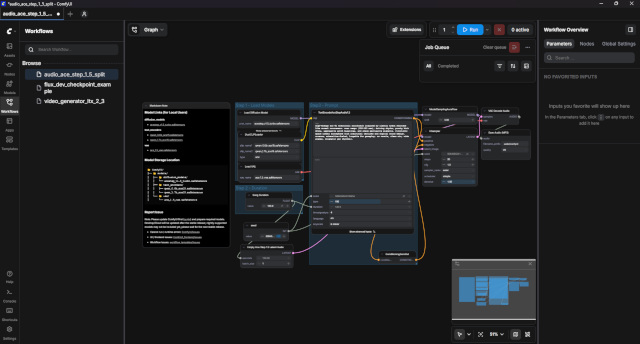
    The easiest way to run ACE-Step-1.5 is to use a ready-made audio generation template. Just search for music text to audio in the workflows window and install.

    Write a prompt describing the genre and mood (for example, “uplifting synthwave track with heavy bass”) in the `Prompt Input` node. Specify the desired duration and press RUN.
    The first generation may take time, as the models will be loaded into the video card memory and process complex acoustic patterns.

    https://github.com/comfyanonymous/ComfyUI
    https://www.youtube.com/watch?v=UAlLD5fS7-c

    Raspberry PI 3 as a Wi-Fi router

    There are a lot of articles on the Internet on how to make a Wi-Fi router from a Raspberry Pi (RPI), in this post I will briefly describe my method of creating a Wi-Fi router with a sing-box on board. The described method works at the current time, and a lot may change in the future. So use this note as a rough overview of what you’ll be up against.

    SSH

    For those who do not know how to work with OpenWrt, I recommend installing dietPI.
    Connect RPI to your current router via eth0, then connect there via SSH. You can find out the RPI IP address in the dhcp panel of the router. Connect directly to root, for example like this:

    ssh root@[IP_ADDRESS]
    

    Access point

    The default dietPI password for root is dietpi. Once connected, you will be greeted by the dietPI installer/configurator. When finished, you will need to connect again due to the device rebooting.

    First, you need to configure hostapd so that devices can see your access point. If hostapd is not installed, then install it via apt.

    Next you will need to write a config for hostapd. Example of my config:

    interface=wlan0
    driver=nl80211
    ssid=MyPiAP
    hw_mode=a
    channel=157
    wmm_enabled=1
    
    auth_algs=1
    wpa=2
    wpa_passphrase=your_password
    wpa_key_mgmt=WPA-PSK
    rsn_pairwise=CCMP
    ieee80211n=1
    ieee80211ac=0
    ieee80211ax=0
    country_code=RU
    

    The meaning of the hostapd config can be found in the manual. However, what is important is to configure it for yourself – the channel (2.4GHz or 5GHz), the country code, otherwise without this your localized devices can work with the access point correctly, I have already done this and know, so be sure to set your country.

    DHCP

    Next, install and configure dnsmasq to implement DHCP. This is necessary for the connected computers to determine the IP address and DNS server.
    Example of my config:

    interface=wlan0
    dhcp-range=172.19.0.10,172.19.0.200,255.255.255.0,12h
    
    dhcp-option=3,172.19.0.1
    
    dhcp-option=6,1.1.1.1,8.8.8.8
    
    no-resolv
    
    server=1.1.1.1
    server=8.8.8.8
    

    This is the minimum config that will allow you to connect to an access point and get an IP address. Next you will need to configure routing and NAT. This is necessary so that connected computers can access the Internet.

    Here the note goes into the category of typical routing setup on a regular Debian compatible system, about which there are a lot of articles on the Internet. Then it all depends on what goals you are pursuing, for example, connecting to an external server as a new interface in the system, or just doing wlan0 <-> eth0, this is where the RPI specifics end, then configure it to your taste.

    I would also like to mention the need to configure custom system services via systemctl; there may be a need to connect services in a chain; all this is in the systemctl manuals on the network. If there are problems at the service level, then check the logs in journalctl.

    Wi-Fi adapter

    The built-in RPI3 turned out to be frankly weak and does not support 5GHz. Therefore, I connected the RITMIX RWA-150 adapter on the Realtek RTL8811CU chipset via USB 2. The drivers were added to the Linux kernel which was in my dietPi version. Next, using dietpi-config, I turned off the built-in Wi-Fi completely. As a result, there was only one wlan0 USB adapter left.

    Conclusion

    From the speed measurements, we were able to squeeze out about 50Mbps from RPI3 over Wi-Fi (after connecting a 5GHz adapter), which means a loss of half the speed compared to connecting directly to the router. I admit that more productive RPI models will allow you to achieve better results, also specialized OpenWrt devices and ready-made solutions may be better for your needs.

    Sources

    https://forums.raspberrypi.com/viewtopic.php?t=394710
    https://superuser.com/questions/1408586/raspberry-pi-wifi-hotspot-slow-internet-speed
    https://www.youtube.com/watch?v=jlHWnKVpygw

    Local image generation: ComfyUI and FLUX model

    Nowadays, you don’t have to rely on cloud services: you can generate high-quality images entirely on your own hardware. In this post, I will describe how to run the modern FLUX model locally on your computer using ComfyUI.

    ComfyUI uses node-based architecture. This allows you to:
    – Totally control every stage of generation.
    – Easily share ready-made “workflows”

    FLUX is a large model, so the hardware requirements are higher than SD 1.5 or SDXL:
    Video card (GPU): Nvidia RTX with 12 GB VRAM or higher (for comfortable work). If you have 8 GB or less, you will have to use the quantized versions (GGUF or NF4).
    Random access memory (RAM): minimum 16 GB (preferably 32 GB and above).
    Disk Space: Approximately 20–50 GB for models and components.

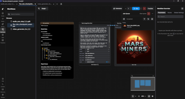
    The easiest way to start FLUX is to use a ready-made template. Just search for flux text to image in the workflows window and install.

    Write a prompt in English in the `Text to Image (Flux.1 Dev)` node, select the resolution (FLUX works well with 1024×1024 and even higher) and press RUN.

    The first generation may take time as the models will be loaded into the video card memory.

    https://github.com/comfyanonymous/ComfyUI

    Running macOS in Docker

    It is possible to run macOS in Docker, despite the objections of people who say that this is impossible, and supposedly macOS has some kind of protection systems that can resist this.

    Some of the classic ways to run macOS on PC machines have historically been:
    *Hackintosh
    * Virtualization, for example using VMWare

    Hackintosh assumes the presence of hardware similar or very close to the original Mac. Virtualization imposes certain requirements on hardware, but generally not as strict as in the case of Hackintosh. However, in the case of virtualization, there are performance problems, since macOS is not optimized for working in a virtual environment.

    Recently, it has become possible to run macOS in Docker. This is made possible by the Docker-OSX project, which provides ready-made macOS images to run on Docker. It is worth noting that Docker-OSX is not an official Apple project and is not supported by it. However, it allows you to run macOS on Docker and use it to develop and test applications.

    One of the first projects to run macOS in Docker:
    https://github.com/sickcodes/Docker-OSX

    However, I was never able to launch it fully; after loading into Recovery OS, my keyboard and mouse simply fell off, and I could not continue the installation. At the same time, in the first boot menu, the keyboard works. Perhaps the fact is that this project is no longer so actively supported, and there are some specific problems when running on Windows 11 + WSL2 + Ubuntu.

    One of the most active projects at the moment:
    https://github.com/dockur/macos

    Allows you to run macOS in Docker, the interface works through the browser via VNC(?) forwarding. After startup, macOS is available at http://localhost:5900

    I managed to run this project and install macOS Big Sur (minute 2020) on Windows 11 + WSL2 + Ubuntu, but only by changing the compose file, namely:

    environment:
        VERSION: "11"
        RAM_SIZE: "8G"
        CPU_CORES: "4"
    

    VERSION: “11” is the version of macOS, in this case Big Sur
    RAM_SIZE: “8G” is the amount of RAM allocated for macOS
    CPU_CORES: “4” is the number of CPU cores allocated to macOS

    At the moment, running macOS tahoe (16) is also possible, but there are a number of problems that the project developers are trying to solve valiantly.

    This original way of launching macOS allows you to try it on your non-Mac hardware and, having suffered enough, go and buy yourself a Mac. However, it can be useful for testing software on older systems and general development.

    Building Swift in WSL2 (Linux)

    The Swift ecosystem is actively developing outside of Apple platforms, and today it is quite comfortable to write in it under Windows using the Windows Subsystem for Linux (WSL2). It is worth considering that for assemblies under Linux/WSL, a lightweight version of Swift is available – without proprietary Apple frameworks (such as SwiftUI, UIKit, AppKit, CoreData, CoreML, ARKit, SpriteKit and other iOS/macOS-specific libraries), but for console utilities and the backend this is more than enough. In this post, we will walk through the process of preparing the environment and building the Swift compiler from source code inside WSL2 step by step (using Ubuntu/Debian as an example).

    We update the list of packages and the system itself:

    sudo apt update && sudo apt upgrade -y
    

    Install the necessary dependencies for the build:

    sudo apt install -y \
      git cmake ninja-build clang python3 python3-pip \
      libicu-dev libxml2-dev libcurl4-openssl-dev \
      libedit-dev libsqlite3-dev swig libncurses5-dev \
      pkg-config tzdata rsync
    

    Install the compiler and linker (LLVM and LLD):

    sudo apt install -y llvm lld
    

    Clone the Swift repository with all dependencies:

    git clone https://github.com/apple/swift.git
    cd swift
    utils/update-checkout --clone
    

    Install `swiftly` and ready-made swift with swiftc

    curl -O https://download.swift.org/swiftly/linux/swiftly-$(uname -m).tar.gz && \
    tar zxf swiftly-$(uname -m).tar.gz && \
    ./swiftly init --quiet-shell-followup && \
    . "${SWIFTLY_HOME_DIR:-$HOME/.local/share/swiftly}/env.sh" && \
    hash -r
    

    Let’s start the build (this will take a long time):

    utils/build-script \
      --release-debuginfo \
      --swift-darwin-supported-archs="x86_64" \
      --llvm-targets-to-build="X86" \
      --skip-build-benchmarks \
      --skip-test-cmark \
      --skip-test-swift \
      --skip-ios \
      --skip-tvos \
      --skip-watchos \
      --skip-build-libdispatch=false \
      --skip-build-cmark=false \
      --skip-build-foundation \
      --skip-build-lldb \
      --skip-build-xctest \
      --skip-test-swift
    

    After the build is complete, add the path to the compiler to PATH (specify your path to the build folder):

    export PATH=/root/Sources/3rdparty/build/Ninja-RelWithDebInfoAssert/swift-linux-x86_64/bin/swiftc:$PATH
    

    We check that the installed version of Swift is working:

    swift --version
    

    Create a test file and run it:

    echo "print(\"Hello, World!\")" > hello.swift
    swift hello.swift
    

    You can also compile the binary and run it:

    swiftc hello.swift
    ./hello
    

    Sources

    Pattern Interpreter in practice

    In last article we looked at the theory of the Interpreter pattern, learned what an AST tree is and how to abstract terminal and non-terminal expressions. This time, let’s step away from the theory and see how this pattern is applied in serious commercial projects that we all use every day!

    Spoiler: You may be using the Interpreter pattern right now, just by reading this text in your browser!

    One of the most striking and, perhaps, the most important examples of the use of this pattern in the industry is JavaScript. The language, which was originally created “on the knee,” today works on billions of devices precisely thanks to the concept of interpretation.

    10 days that changed the Internet

    The history of JavaScript is full of legends. In 1995, Brendan Eich, while working at Netscape Communications, was given the task of creating a simple scripting language that could run directly in a browser (Netscape Navigator) to make web pages interactive. Management wanted something with a syntax similar to the then super popular Java, but intended not for professional engineers, but for web designers.

    Eich had only 10 days to write the first prototype of the language, which was then called Mocha (then LiveScript, and only then JavaScript for marketing reasons). The rush was not accidental: Microsoft was hot on its heels, which at the same time was actively preparing its own scripting language VBScript for embedding in the Internet Explorer browser. Netscape urgently needed to release its response so as not to lose in the looming browser war.

    There was simply no time to write a complex compiler into machine code. The obvious and fastest solution for Eich was the architecture of the classic Interpreter.

    The first interpreter (SpiderMonkey) worked like this:

    1. It read the text source code of the script from the page.
    2. The lexical analyzer broke the text into tokens.
    3. The parser built an Abstract Syntax Tree (AST). In terms of the Interpreter pattern, this tree consisted of terminal expressions (strings, numbers like 42) and non-terminal (function calls, statements like If, ​​While).
    4. Then the virtual machine “traversed” this tree step by step, executing the instructions embedded in it at each node (calling a method similar to Interpret()).

    Context and Objects

    Remember the Context object that we had to pass to the Interpret(Context context) method in the classic implementation? The interpreter needs it to store the current memory state.

    In the case of JavaScript, the role of this context at the top level is played by a Global object (for example, window in a browser). When your AST node tries to, say, write text to the screen via document.write(“Hello”), the interpreter accesses its context (the document object) and calls the desired internal browser API.

    It is thanks to the interpreter that JavaScript is able to interact so easily with the DOM (Document Object Model) – these are all just objects in a context that are accessed by tree nodes.

    Evolution of the interpreter: JIT Compilation

    Historically, JS in browsers has long remained a “pure” interpreter. And this had a big disadvantage – slow speed. Parsing the tree and slowly traversing each node each time the script was executed slowed down complex web applications.

    With the advent of Google’s V8 engine (built into Chrome) in 2008, a revolution occurred. Engineers realized that one interpreter is not enough for the modern web. The engine has become more complex: it still builds the AST tree, but now uses JIT (Just-In-Time) compilation.

    Modern JS engines (V8, SpiderMonkey) work like a complex pipeline:

    1. The fast and dumb base interpreter starts executing your JS code instantly, without even waiting for it to compile (the classic pattern still works here).
    2. In parallel, the engine monitors “hot” sections of code (loops or functions that are called thousands of times).
    3. These sections are compiled by the JIT compiler directly into optimized machine code, bypassing the slow interpreter.

    It was this combination of the instant start of the interpreter and the computing power of compilation that allowed JavaScript to take over the world, becoming the language of servers (Node.js) and mobile applications (React Native).

    Interpreter in the gaming industry

    Despite the dominance of C++ in heavy computing, the Interpreter pattern is an industry standard in game development for creating game logic. For what? So that game designers can make games without the risk of “dropping” the engine or the need to constantly recompile it.

    An excellent historical example is UnrealScript – the language in which the logic of the Unreal Tournament and Gears of War games was written in Unreal Engine 1, 2 and 3. The text was compiled into compact abstract machine bytecode, which was then step by step (interpreted) by the engine’s virtual machine.

    Visual graph scripts (Blueprints)

    Today, text has been replaced by visual programming – the Blueprints system in Unreal Engine 4 and 5.

    If you’ve ever opened a Blueprint in Unreal Engine, you’ve seen a lot of Nodes connected by wires. Architecturally, the entire Blueprints graph is a huge Abstract Syntax Tree (AST) drawn on the screen:

    1. Terminal Expressions: Constant nodes. For example, a node that simply stores the number 42 or a string. They return a specific value when interpreted.
    2. Non-Terminal Expressions: Compute nodes (Add) or flow control nodes (Branch). They have argument inputs, which the interpreter first evaluates recursively before producing the result as an output pin.

    And the role of context here is played by the memory of an instance of a specific game object (Actor). The Interpreter Machine safely “walks” through this graph, requesting data and performing transitions.

    Where else is the Interpreter used?

    The interpreter pattern can be found in almost any complex system where dynamic instructions need to be executed. Here are just a few examples from commercial software:

    • Interpreted programming languages ​​(Python, Ruby, PHP). Their entire runtime is based on the classic pattern. For example, the CPython reference implementation first parses your .py script into an AST, compiles it into bytecode, and then a huge virtual machine (compute loop) interprets that bytecode step by step.
    • Java Virtual Machine (JVM). Initially, Java code is compiled not into machine instructions, but into bytecode. When you run the application, the JVM acts as an interpreter (albeit with aggressive JIT compilation, just like in V8).
    • Databases and SQL When you issue an SQL query (SELECT * FROM users) in PostgreSQL or MySQL, the database engine acts as an interpreter. It performs lexical analysis, builds an AST query tree, generates an execution plan, and then literally “interprets” this plan by iterating over the rows of the tables.
    • Regular expressions (RegEx). Any regular expression engine internally parses a string pattern (for example, ^\d{3}-\d{2}$) into a state graph (NFA/DFA Automata), which the internal interpreter then passes through, matching each input character with the vertices of this graph.
    • Unity Shader Graph / Unreal Material Editor – interpret visual nodes into modular shader code (GLSL/HLSL).
    • Blender Geometry Nodes – interpret mathematical and geometric operations to procedurally generate 3D models in real time.

    Total

    The Interpreter pattern has long gone beyond the scope of “writing your own calculator”. This is the most powerful industry standard. From JavaScript engines that execute gigabytes of code behind the scenes of browsers every day, to game designers that allow you to build complex logic without knowledge of C++, interpreters remain one of the most important architectural concepts in modern IT development.

    ollama-call

    If you use Ollama and don’t want to write your own API wrapper every time,
    the ollama_call project significantly simplifies the work.

    This is a small Python library that allows you to send a request to a local LLM with one function
    and immediately receive a response, including in JSON format.

    Installation

    pip install ollama-call
    

    Why is it needed

    • minimal code for working with the model;
    • structured JSON response for further processing;
    • convenient for rapid prototypes and MVPs;
    • supports streaming output if necessary.

    Use example

    from ollama_call import ollama_call
    
    response = ollama_call(
        user_prompt="Hello, how are you?",
        format="json",
        model="gemma3:12b"
    )
    
    print(response)
    

    When it is especially useful

    • you write scripts or services on top of Ollama;
    • need a predictable response format;
    • there is no desire to connect heavy frameworks.

    Total

    ollama_call is a lightweight and clear wrapper for working with Ollama from Python.
    A good choice if simplicity and quick results are important.

    GitHub
    https://github.com/demensdeum/ollama_call

    SFAP: a modular framework for modern data acquisition and processing

    In the context of the active development of automation and artificial intelligence, the task of effectively collecting,
    Cleaning and transforming data becomes critical. Most solutions only close
    separate stages of this process, requiring complex integration and support.

    SFAP (Seek · Filter · Adapt · Publish) is an open-source project in Python,
    which offers a holistic and extensible approach to processing data at all stages of its lifecycle:
    from searching for sources to publishing the finished result.

    What is SFAP

    SFAP is an asynchronous framework built around a clear concept of a data processing pipeline.
    Each stage is logically separate and can be independently expanded or replaced.

    The project is based on the Chain of Responsibility architectural pattern, which provides:

    • pipeline configuration flexibility;
    • simple testing of individual stages;
    • scalability for high loads;
    • clean separation of responsibilities between components.

    Main stages of the pipeline

    Seek – data search

    At this stage, data sources are discovered: web pages, APIs, file storages
    or other information flows. SFAP makes it easy to connect new sources without changing
    the rest of the system.

    Filter – filtering

    Filtering is designed to remove noise: irrelevant content, duplicates, technical elements
    and low quality data. This is critical for subsequent processing steps.

    Adapt – adaptation and processing

    The adaptation stage is responsible for data transformation: normalization, structuring,
    semantic processing and integration with AI models (including generative ones).

    Publish – publication

    At the final stage, the data is published in the target format: databases, APIs, files, external services
    or content platforms. SFAP does not limit how the result is delivered.

    Key features of the project

    • Asynchronous architecture based on asyncio
    • Modularity and extensibility
    • Support for complex processing pipelines
    • Ready for integration with AI/LLM solutions
    • Suitable for highly loaded systems

    Practical use cases

    • Aggregation and analysis of news sources
    • Preparing datasets for machine learning
    • Automated content pipeline
    • Cleansing and normalizing large data streams
    • Integration of data from heterogeneous sources

    Getting started with SFAP

    All you need to get started is:

    1. Clone the project repository;
    2. Install Python dependencies;
    3. Define your own pipeline steps;
    4. Start an asynchronous data processing process.

    The project is easily adapted to specific business tasks and can grow with the system,
    without turning into a monolith.

    Conclusion

    SFAP is not just a parser or data collector, but a full-fledged framework for building
    modern data-pipeline systems. It is suitable for developers and teams who care about
    scalable, architecturally clean, and data-ready.
    The project source code is available on GitHub:
    https://github.com/demensdeum/SFAP

    Why can’t I fix the bug?

    You spend hours working on the code, going through hypotheses, adjusting the conditions, but the bug is still reproduced. Sound familiar? This state of frustration is often called “ghost hunting.” The program seems to live its own life, ignoring your corrections.

    One of the most common – and most annoying – reasons for this situation is looking for an error in completely the wrong place in the application.

    The trap of “false symptoms”

    When we see an error, our attention is drawn to the place where it “shot”. But in complex systems, where a bug occurs (crash or incorrect value) is only the end of a long chain of events. When you try to fix the ending, you are fighting the symptoms, not the disease.

    This is where the flowchart concept comes in.

    How it works in reality

    Of course, it is not necessary to directly draw (draw) a flowchart on paper every time, but it is important to have it in your head or at hand as an architectural guide. A flowchart allows you to visualize the operation of an application as a tree of outcomes.

    Without understanding this structure, the developer is often groping in the dark. Imagine the situation: you edit the logic in one condition branch, while the application (due to a certain set of parameters) goes to a completely different branch that you didn’t even think about.

    Result: You spend hours on a “perfect” code fix in one part of the algorithm, which, of course, does nothing to fix the problem in another part of the algorithm where it actually fails.


    Algorithm for defeating a bug

    To stop beating on a closed door, you need to change your approach to diagnosis:

    • Find the state in the outcome tree:Before writing code, you need to determine exactly the path that the application has taken. At what point did logic take a wrong turn? What specific state (State) led to the problem?
    • Reproduction is 80% of success: This is usually done by testers and automated tests. If the bug is “floating”, development is involved in the process to jointly search for conditions.
    • Use as much information as possible: Logs, OS version, device parameters, connection type (Wi-Fi/5G) and even a specific telecom operator are important for localization.

    “Photograph” of the moment of error

    Ideally, to fix it, you need to get the full state of the application at the time the bug was reproduced. Interaction logs are also critically important: they show not only the final point, but also the entire user path (what actions preceded the failure). This helps to understand how to recreate a similar state again.

    Future tip: If you encounter a complex case, add extended debug logging information to this section of code in case the situation happens again.


    The problem of “elusive” states in the era of AI

    In modern systems using LLM (Large Language Models), classical determinism (“one input, one output”) is often violated. You can pass exactly the same input data, but get a different result.

    This happens due to the non-determinism of modern production systems:

    • GPU Parallelism: GPU floating point operations are not always associative. Due to parallel execution of threads, the order in which numbers are added may change slightly, which may affect the result.
    • GPU temperature and throttling: Execution speed and load distribution may depend on the physical state of the hardware. In huge models, these microscopic differences accumulate and can lead to the selection of a different token at the output.
    • Dynamic batching: In the cloud, your request is combined with others. Different batch sizes change the mathematics of calculations in the kernels.

    Under such conditions, it becomes almost impossible to reproduce “that same state”. Only a statistical approach to testing can save you here.


    When logic fails: Memory problems

    If you are working with “unsafe” languages ​​(C or C++), the bug may occur due to Memory Corruption.

    These are the most severe cases: an error in one module can “overwrite” data in another. This leads to completely inexplicable and isolated failures that cannot be traced using normal application logic.

    How to protect yourself at the architectural level?

    To avoid such “mystical” bugs, you should use modern approaches:

    • Multithreaded programming patterns:Clear synchronization eliminates race conditions.
    • Thread-safe languages: Tools that guarantee memory safety at compile time:
      • Rust: Ownership system eliminates memory errors.
      • Swift 6 Concurrency:Strong data isolation checks.
      • Erlang: Complete process isolation through the actor model.

    Summary

    Fixing a bug is not about writing new code, but about understanding how the old one works. Remember: you could be wasting time editing a branch that management doesn’t even touch. Record the state of the system, take into account the factor of AI non-determinism and choose safe tools.

    Block diagrams in practice without formalin

    The block diagram is a visual tool that helps to turn a complex algorithm into an understandable and structured sequence of actions. From programming to business process management, they serve as a universal language for visualization, analysis and optimization of the most complex systems.

    Imagine a map where instead of roads is logic, and instead of cities – actions. This is a block diagram-an indispensable tool for navigation in the most confusing processes.

    Example 1: Simplified game launching scheme
    To understand the principle of work, let’s present a simple game launch scheme.

    This scheme shows the perfect script when everything happens without failures. But in real life, everything is much more complicated.

    Example 2: Expanded scheme for starting the game with data loading
    Modern games often require Internet connection to download user data, saving or settings. Let’s add these steps to our scheme.

    This scheme is already more realistic, but what will happen if something goes wrong?

    How was it: a game that “broke” with the loss of the Internet

    At the start of the project, developers could not take into account all possible scenarios. For example, they focused on the main logic of the game and did not think what would happen if the player has an Internet connection.

    In such a situation, the block diagram of their code would look like this:

    In this case, instead of issuing an error or closing correctly, the game froze at the stage of waiting for data that she did not receive due to the lack of a connection. This led to the “black screen” and freezing the application.

    How it became: Correction on user complaints

    After numerous users’ complaints about hovering, the developer team realized that we needed to correct the error. They made changes to the code by adding an error processing unit that allows the application to respond correctly to the lack of connection.

    This is what the corrected block diagram looks like, where both scenarios are taken into account:

    Thanks to this approach, the game now correctly informs the user about the problem, and in some cases it can even go to offline mode, allowing you to continue the game. This is a good example of why block diagrams are so important : they make the developer think not only about the ideal way of execution, but also about all possible failures, making the final product much more stable and reliable.

    Uncertain behavior

    Hanging and errors are just one examples of unpredictable behavior of the program. In programming, there is a concept of uncertain behavior (undefined behavior) – this is a situation where the standard of the language does not describe how the program should behave in a certain case.

    This can lead to anything: from random “garbage” in the withdrawal to the failure of the program or even serious security vulnerability. Indefinite behavior often occurs when working with memory, for example, with lines in the language of C.

    An example from the language C:

    Imagine that the developer copied the line into the buffer, but forgot to add to the end the zero symbol (`\ 0`) , which marks the end of the line.

    This is what the code looks like:

    #include 
    
    int main() {
    char buffer[5];
    char* my_string = "hello";
    
    memcpy(buffer, my_string, 5);
    
    printf("%s\n", buffer);
    return 0;
    }
    

    Expected result: “Hello”
    The real result is unpredictable.

    Why is this happening? The `Printf` function with the specifier`%S` expects that the line ends with a zero symbol. If he is not, she will continue to read the memory outside the highlighted buffer.

    Here is the block diagram of this process with two possible outcomes:

    This is a clear example of why the block diagrams are so important: they make the developer think not only about the ideal way of execution, but also about all possible failures, including such low-level problems, making the final product much more stable and reliable.

    Pixel Perfect: myth or reality in the era of declarativeness?

    In the world of interfaces development, there is a common concept – “Pixel Perfect in the Lodge” . It implies the most accurate reproduction of the design machine to the smallest pixel. For a long time it was a gold standard, especially in the era of a classic web design. However, with the arrival of the declarative mile and the rapid growth of the variety of devices, the principle of “Pixel Perfect” is becoming more ephemeral. Let’s try to figure out why.

    Imperial Wysiwyg vs. Declarative code: What is the difference?

    Traditionally, many interfaces, especially desktop, were created using imperative approaches or Wysiwyg (What You See is What You Get) of editors. In such tools, the designer or developer directly manipulates with elements, placing them on canvas with an accuracy to the pixel. It is similar to working with a graphic editor – you see how your element looks, and you can definitely position it. In this case, the achievement of “Pixel Perfect” was a very real goal.

    However, modern development is increasingly based on declarative miles . This means that you do not tell the computer to “put this button here”, but describe what you want to get. For example, instead of indicating the specific coordinates of the element, you describe its properties: “This button should be red, have 16px indentations from all sides and be in the center of the container.” Freimvorki like React, Vue, Swiftui or Jetpack Compose just use this principle.

    Why “Pixel Perfect” does not work with a declarative mile for many devices

    Imagine that you create an application that should look equally good on the iPhone 15 Pro Max, Samsung Galaxy Fold, iPad Pro and a 4K resolution. Each of these devices has different screen resolution, pixel density, parties and physical sizes.

    When you use the declarative approach, the system itself decides how to display your described interface on a particular device, taking into account all its parameters. You set the rules and dependencies, not harsh coordinates.

    * Adaptability and responsiveness: The main goal of the declarative miles is to create adaptive and responsive interfaces . This means that your interface should automatically adapt to the size and orientation of the screen without breaking and maintaining readability. If we sought to “Pixel Perfect” on each device, we would have to create countless options for the same interface, which will completely level the advantages of the declarative approach.
    * Pixel density (DPI/PPI): The devices have different pixel density. The same element with the size of 100 “virtual” pixels on a device with high density will look much smaller than on a low -density device, if you do not take into account the scaling. Declarative frameworks are abstracted by physical pixels, working with logical units.
    * Dynamic content: Content in modern applications is often dynamic – its volume and structure may vary. If we tattered hard to the pixels, any change in text or image would lead to the “collapse” of the layout.
    * Various platforms: In addition to the variety of devices, there are different operating systems (iOS, Android, Web, Desktop). Each platform has its own design, standard controls and fonts. An attempt to make an absolutely identical, Pixel Perfect interface on all platforms would lead to an unnatural type and poor user experience.

    The old approaches did not go away, but evolved

    It is important to understand that the approach to interfaces is not a binary choice between “imperative” and “declarative”. Historically, for each platform there were its own tools and approaches to the creation of interfaces.

    * Native interface files: for iOS it were XIB/Storyboards, for Android-XML marking files. These files are a Pixel-PERFECT WYSIWYG layout, which is then displayed in the radio as in the editor. This approach has not disappeared anywhere, it continues to develop, integrating with modern declarative frames. For example, Swiftui in Apple and Jetpack Compose in Android set off on the path of a purely declarative code, but at the same time retained the opportunity to use a classic layout.
    * hybrid solutions: Often in real projects, a combination of approaches is used. For example, the basic structure of the application can be implemented declaratively, and for specific, requiring accurate positioning of elements, lower -level, imperative methods can be used or native components developed taking into account the specifics of the platform.

    from monolith to adaptability: how the evolution of devices formed a declarative mile

    The world of digital interfaces has undergone tremendous changes over the past decades. From stationary computers with fixed permits, we came to the era of exponential growth of the variety of user devices . Today, our applications should work equally well on:

    * smartphones of all form factors and screen sizes.
    * tablets with their unique orientation modes and a separated screen.
    * laptops and desktops with various permits of monitors.
    * TVs and media centers , controlled remotely. It is noteworthy that even for TVs, the remarks of which can be simple as Apple TV Remote with a minimum of buttons, or vice versa, overloaded with many functions, modern requirements for interfaces are such that the code should not require specific adaptation for these input features. The interface should work “as if by itself”, without an additional description of what “how” to interact with a specific remote control.
    * smart watches and wearable devices with minimalistic screens.
    * Virtual reality helmets (VR) , requiring a completely new approach to a spatial interface.
    * Augmented reality devices (AR) , applying information on the real world.
    * automobile information and entertainment systems .
    * And even household appliances : from refrigerators with sensory screens and washing machines with interactive displays to smart ovens and systems of the Smart House.

    Each of these devices has its own unique features: physical dimensions, parties ratio, pixel density, input methods (touch screen, mouse, controllers, gestures, vocal commands) and, importantly, the subtleties of the user environment . For example, a VR shlesh requires deep immersion, and a smartphone-fast and intuitive work on the go, while the refrigerator interface should be as simple and large for quick navigation.

    Classic approach: The burden of supporting individual interfaces

    In the era of the dominance of desktops and the first mobile devices, the usual business was the creation and support of of individual interface files or even a completely separate interface code for each platform .

    * Development under iOS often required the use of Storyboards or XIB files in XCode, writing code on Objective-C or SWIFT.
    * For Android the XML marking files and the code on Java or Kotlin were created.
    * Web interfaces turned on HTML/CSS/JavaScript.
    * For C ++ applications on various desktop platforms, their specific frameworks and tools were used:
    * In Windows these were MFC (Microsoft Foundation Classes), Win32 API with manual drawing elements or using resource files for dialog windows and control elements.
    * Cocoa (Objective-C/Swift) or the old Carbon API for direct control of the graphic interface were used in macos .
    * In linux/unix-like systems , libraries like GTK+ or QT were often used, which provided their set of widgets and mechanisms for creating interfaces, often via XML-like marking files (for example, .ui files in Qt Designer) or direct software creation of elements.

    This approach ensured maximum control over each platform, allowing you to take into account all its specific features and native elements. However, he had a huge drawback: duplication of efforts and tremendous costs for support . The slightest change in design or functionality required the introduction of a right to several, in fact, independent code bases. This turned into a real nightmare for developer teams, slowing down the output of new functions and increasing the likelihood of errors.

    declarative miles: a single language for diversity

    It was in response to this rapid complication that the declarative miles appeared as the dominant paradigm. Framws like react, vue, swiftui, jetpack compose and others are not just a new way of writing code, but a fundamental shift in thinking.

    The main idea of the declarative approach : Instead of saying the system “how” to draw every element (imperative), we describe “what“ we want to see (declarative). We set the properties and condition of the interface, and the framework decides how to best display it on a particular device.

    This became possible thanks to the following key advantages:

    1. Abstraction from the details of the platform: declarative fraimvorki are specially designed to forget about low -level details of each platform. The developer describes the components and their relationships at a higher level of abstraction, using a single, transferred code.
    2. Automatic adaptation and responsiveness: Freimvorki take responsibility for automatic scaling, changing the layout and adaptation of elements to different sizes of screens, pixel density and input methods. This is achieved through the use of flexible layout systems, such as Flexbox or Grid, and concepts similar to “logical pixels” or “DP”.
    3. consistency of user experience: Despite the external differences, the declarative approach allows you to maintain a single logic of behavior and interaction throughout the family of devices. This simplifies the testing process and provides more predictable user experience.
    4. Acceleration of development and cost reduction: with the same code capable of working on many platforms, significantly is reduced by the time and cost of development and support . Teams can focus on functionality and design, and not on repeated rewriting the same interface.
    5. readiness for the future: the ability to abstract from the specifics of current devices makes the declarative code more more resistant to the emergence of new types of devices and form factors . Freimvorki can be updated to support new technologies, and your already written code will receive this support is relatively seamless.

    Conclusion

    The declarative mile is not just a fashion trend, but the necessary evolutionary step caused by the rapid development of user devices, including the sphere of the Internet of things (IoT) and smart household appliances. It allows developers and designers to create complex, adaptive and uniform interfaces, without drowning in endless specific implementations for each platform. The transition from imperative control over each pixel to the declarative description of the desired state is a recognition that in the world of the future interfaces should be flexible, transferred and intuitive regardless of which screen they are displayed.

    Programmers, designers and users need to learn how to live in this new world. The extra details of the Pixel Perfect, designed to a particular device or resolution, lead to unnecessary time costs for development and support. Moreover, such harsh layouts may simply not work on devices with non-standard interfaces, such as limited input TVs, VR and AR shifts, as well as other devices of the future, which we still do not even know about today. Flexibility and adaptability – these are the keys to the creation of successful interfaces in the modern world.

    Why do programmers do nothing even with neural networks

    Today, neural networks are used everywhere. Programmers use them to generate code, explain other solutions, automate routine tasks, and even create entire applications from scratch. It would seem that this should lead to an increase in efficiency, reducing errors and acceleration of development. But reality is much more prosaic: many still do not succeed. The neural networks do not solve key problems – they only illuminate the depth of ignorance.

    full dependence on LLM instead of understanding

    The main reason is that many developers are completely relying on LLM, ignoring the need for a deep understanding of the tools with which they work. Instead of studying documentation – a chat request. Instead of analyzing the reasons for the error – copying the decision. Instead of architectural solutions – the generation of components according to the description. All this can work at a superficial level, but as soon as a non -standard task arises, integration with a real project or the need for fine tuning is required, everything is crumbling.

    Lack of context and outdated practices

    The neural networks generate the code generalized. They do not take into account the specifics of your platform, version of libraries, environmental restrictions or architectural solutions of the project. What is generated often looks plausible, but has nothing to do with the real, supported code. Even simple recommendations may not work if they belong to the outdated version of the framework or use approaches that have long been recognized as ineffective or unsafe. Models do not understand the context – they rely on statistics. This means that errors and antipattterns, popular in open code, will be reproduced again and again.

    redundancy, inefficiency and lack of profiling

    The code generated AI is often redundant. It includes unnecessary dependencies, duplicates logic, adds abstractions unnecessarily. It turns out an ineffective, heavy structure that is difficult to support. This is especially acute in mobile development, where the size of the gang, response time and energy consumption are critical.

    The neural network does not conduct profiling, does not take into account the restrictions of the CPU and GPU, does not care about the leaks of memory. It does not analyze how effective the code is in practice. Optimization is still handmade, requiring analysis and examination. Without it, the application becomes slow, unstable and resource -intensive, even if they look “right” from the point of view of structure.

    Vulnerability and a threat to security

    Do not forget about safety. There are already known cases when projects partially or fully created using LLM were successfully hacked. The reasons are typical: the use of unsafe functions, lack of verification of input data, errors in the logic of authorization, leakage through external dependencies. The neural network can generate a vulnerable code simply because it was found in open repositories. Without the participation of security specialists and a full -fledged revision, such errors easily become input points for attacks.

    The law is pareto and the essence of the flaws

    Pareto law works clearly with neural networks: 80% of the result is achieved due to 20% of effort. The model can generate a large amount of code, create the basis of the project, spread the structure, arrange types, connect modules. However, all this can be outdated, incompatible with current versions of libraries or frameworks, and require significant manual revision. Automation here works rather as a draft that needs to be checked, processed and adapted to specific realities of the project.

    Caution optimism

    Nevertheless, the future looks encouraging. Constant updating of training datasets, integration with current documentation, automated architecture checks, compliance with design and security patterns – all this can radically change the rules of the game. Perhaps in a few years we can really write the code faster, safer and more efficiently, relying on LLM as a real technical co -author. But for now – alas – a lot has to be checked, rewritten and modified manually.

    Neural networks are a powerful tool. But in order for him to work for you, and not against you, you need a base, critical thinking and willingness to take control at any time.

    Vibe-core tricks: why LLM still does not work with Solid, Dry and Clean

    With the development of large language models (LLM), such as ChatGPT, more and more developers use them to generate code, design architecture and accelerate integration. However, with practical application, it becomes noticeable: the classical principles of architecture – Solid, Dry, Clean – get along poorly with the peculiarities of the LLM codgendation.

    This does not mean that the principles are outdated – on the contrary, they work perfectly with manual development. But with LLM the approach has to be adapted.

    Why llm cannot cope with architectural principles

    encapsulation

    Incapsulation requires understanding the boundaries between parts of the system, knowledge about the intentions of the developer, as well as follow strict access restrictions. LLM often simplifies the structure, make fields public for no reason or duplicate the implementation. This makes the code more vulnerable to errors and violates the architectural boundaries.

    Abstracts and interfaces

    Design patterns, such as an abstract factory or strategy, require a holistic view of the system and understanding its dynamics. Models can create an interface without a clear purpose without ensuring its implementation, or violate the connection between layers. The result is an excess or non -functional architecture.

    Dry (Donolt Repeat Yourself)

    LLM do not seek to minimize the repeating code – on the contrary, it is easier for them to duplicate blocks than to make general logic. Although they can offer refactoring on request, by default models tend to generate “self -sufficient” fragments, even if it leads to redundancy.

    Clean Architecture

    Clean implies a strict hierarchy, independence from frameworks, directed dependence and minimal connectedness between layers. The generation of such a structure requires a global understanding of the system – and LLM work at the level of probability of words, not architectural integrity. Therefore, the code is mixed, with violation of the directions of dependence and a simplified division into levels.

    What works better when working with LLM

    Wet instead of Dry
    The WET (Write EVERYTHING TWICE) approach is more practical in working with LLM. Duplication of code does not require context from the model of retention, which means that the result is predictable and is easier to correctly correct. It also reduces the likelihood of non -obvious connections and bugs.

    In addition, duplication helps to compensate for the short memory of the model: if a certain fragment of logic is found in several places, LLM is more likely to take it into account with further generation. This simplifies accompaniment and increases resistance to “forgetting”.

    Simple structures instead of encapsulation

    Avoiding complex encapsulation and relying on the direct transmission of data between the parts of the code, you can greatly simplify both generation and debugging. This is especially true with a quick iterative development or creation of MVP.

    Simplified architecture

    A simple, flat structure of the project with a minimum amount of dependencies and abstractions gives a more stable result during generation. The model adapts such a code easier and less often violates the expected connections between the components.

    SDK integration – manually reliable

    Most language models are trained on outdated versions of documentation. Therefore, when generating instructions for installing SDK, errors often appear: outdated commands, irrelevant parameters or links to inaccessible resources. Practice shows: it is best to use official documentation and manual tuning, leaving LLM an auxiliary role – for example, generating a template code or adaptation of configurations.

    Why are the principles still work – but with manual development

    It is important to understand that the difficulties from Solid, Dry and Clean concern the codhegeneration through LLM. When the developer writes the code manually, these principles continue to demonstrate their value: they reduce connectedness, simplify support, increase the readability and flexibility of the project.

    This is due to the fact that human thinking is prone to generalization. We are looking for patterns, we bring repeating logic into individual entities, create patterns. Probably, this behavior has evolutionary roots: reducing the amount of information saves cognitive resources.

    LLM act differently: they do not experience loads from the volume of data and do not strive for savings. On the contrary, it is easier for them to work with duplicate, fragmented information than to build and maintain complex abstractions. That is why it is easier for them to cope with the code without encapsulation, with repeating structures and minimal architectural severity.

    Conclusion

    Large language models are a useful tool in development, especially in the early stages or when creating an auxiliary code. But it is important to adapt the approach to them: to simplify the architecture, limit abstraction, avoid complex dependencies and not rely on them when configuring SDK.

    The principles of Solid, Dry and Clean are still relevant-but they give the best effect in the hands of a person. When working with LLM, it is reasonable to use a simplified, practical style that allows you to get a reliable and understandable code that is easy to finalize manually. And where LLM forgets – duplication of code helps him to remember.

    Porting Surreal Engine C++ to WebAssembly

    In this post I will describe how I ported the Surreal Engine game engine to WebAssembly.

    Surreal Engine is a game engine that implements most of the functionality of the Unreal Engine 1 engine, famous games on this engine are Unreal Tournament 99, Unreal, Deus Ex, Undying. It belongs to the classic engines that worked mainly in a single-threaded execution environment.

    My initial idea was to take on a project that I couldn’t complete in any reasonable amount of time, thus showing my Twitch followers that there are projects that even I can’t do. On my very first stream, I suddenly realized that the task of porting Surreal Engine C++ to WebAssembly using Emscripten was doable.

    Surreal Engine Emscripten Demo

    A month later I can show my fork and assembly of the engine on WebAssembly:
    https://demensdeum.com/demos/SurrealEngine/

    The controls are the same as in the original, using the keyboard arrows. Next, I plan to adapt it to mobile controls (touch), add correct lighting and other graphic features of the Unreal Tournament 99 render.

    Where to start?

    The first thing I want to say is that any project can be ported from C++ to WebAssembly using Emscripten, the only question is how complete the functionality will be. Choose a project whose library ports are already available for Emscripten, in the case of Surreal Engine, you are very lucky, because the engine uses the SDL 2, OpenAL libraries – they are both ported to Emscripten. However, Vulkan is used as a graphics API, which is currently not available for HTML5, work is underway to implement WebGPU, but it is also in the draft stage, and it is also unknown how simple the further port from Vulkan to WebGPU will be, after its full standardization. Therefore, I had to write my own basic OpenGL-ES / WebGL renderer for Surreal Engine.

    Building the project

    The build system in Surreal Engine is CMake, which also simplifies porting, since Emscripten provides its own native builders – emcmake, emmake.
    The Surreal Engine port was based on the code of my last game on WebGL/OpenGL ES and C++ called Death-Mask, because of this the development went much easier, all the necessary build flags were with me, code examples.

    One of the most important points in CMakeLists.txt is the build flags for Emscripten, below is an example from the project file:

    
    -s MAX_WEBGL_VERSION=2 \
    
    -s EXCEPTION_DEBUG \
    
    -fexceptions \
    
    --preload-file UnrealTournament/ \
    
    --preload-file SurrealEngine.pk3 \
    
    --bind \
    
    --use-preload-plugins \
    
    -Wall \
    
    -Wextra \
    
    -Werror=return-type \
    
    -s USE_SDL=2 \
    
    -s ASSERTIONS=1 \
    
    -w \
    
    -g4 \
    
    -s DISABLE_EXCEPTION_CATCHING=0 \
    
    -O3 \
    
    --no-heap-copy \
    
    -s ALLOW_MEMORY_GROWTH=1 \
    
    -s EXIT_RUNTIME=1")


    The build script itself:

    
    emmake make -j 16
    
    cp SurrealEngine.data /srv/http/SurrealEngine/SurrealEngine.data
    
    cp SurrealEngine.js /srv/http/SurrealEngine/SurrealEngine.js
    
    cp SurrealEngine.wasm /srv/http/SurrealEngine/SurrealEngine.wasm
    
    cp ../buildScripts/Emscripten/index.html /srv/http/SurrealEngine/index.html
    
    cp ../buildScripts/Emscripten/background.png /srv/http/SurrealEngine/background.png


    Next, we’ll prepare index.html, which includes the project file system preloader. For posting on the web, I used Unreal Tournament Demo version 338. As you can see from the CMake file, the unpacked game folder was added to the build directory and linked as a preload-file for Emscripten.

    Major code changes

    Then it was necessary to change the game loop, you can’t run an infinite loop, it leads to the browser freezing, instead you need to use emscripten_set_main_loop, I wrote about this feature in my 2017 note “Porting SDL C++ game to HTML5 (Emscripten)
    We change the code for the condition for exiting the while loop to if, then we output the main class of the game engine, which contains the game loop, to the global scope, and write a global function that will call the step of the game loop from the global object:

    
    #include <emscripten.h>
    
    Engine *EMSCRIPTEN_GLOBAL_GAME_ENGINE = nullptr;
    
    void emscripten_game_loop_step() {
    
    	EMSCRIPTEN_GLOBAL_GAME_ENGINE->Run();
    
    }
    
    #endif


    After this, you need to make sure that there are no background threads in the application. If there are, then get ready to rewrite them for single-thread execution, or use the phtread library in Emscripten.
    The background thread in Surreal Engine is used to play music, the main thread of the engine receives data about the current track, about the need to play music, or its absence, then the background thread via mutex receives a new state and starts playing new music, or pauses. The background thread is also used to buffer music during playback.
    My attempts to build Surreal Engine under Emscripten with pthread were unsuccessful, because the SDL2 and OpenAL ports were built without pthread support, and I did not want to rebuild them for the sake of music. Therefore, I moved the background music thread functionality to single-thread execution using a loop. Having removed pthread calls from the C++ code, I moved buffering, music playback to the main thread, so that there were no delays, I increased the buffer by several seconds.

    Next I will describe specific implementations of graphics and sound.

    Vulkan is not supported!

    Yes, Vulkan is not supported in HTML5, although all the advertising brochures point out cross-platform and wide support on platforms as the main advantage of Vulkan. For this reason, I had to write my own basic graphics renderer for a simplified type of OpenGL – ES, it is used on mobile devices, sometimes does not contain fashionable features of modern OpenGL, but it is very well transferred to WebGL, this is what Emscripten implements. Writing a basic tile renderer, bsp rendering, for the simplest display of GUI, and drawing models + maps, was possible in two weeks. This was probably the most difficult part of the project. There is still a lot of work ahead to implement the full functionality of the Surreal Engine rendering, so any help from readers in the form of code and pull requests is welcome.

    OpenAL is supported!

    It was a great stroke of luck that Surreal Engine uses OpenAL for audio output. After writing a simple hello world in OpenAL and building it in WebAssembly using Emscripten, it became clear to me how simple it all is, and I set out to port the audio.
    After several hours of debugging, it became obvious that there are several bugs in the OpenAL implementation of Emscripten, for example, when initializing the reading of the number of mono channels, the method returned an infinite number, and after trying to initialize a vector of infinite size, C++ crashes with the exception vector::length_error.
    This was circumvented by hardcoding the number of mono channels to 2048:

    
    		alcGetIntegerv(alDevice, ALC_STEREO_SOURCES, 1, &stereoSources);


    #if __EMSCRIPTEN__
    
    		monoSources = 2048; // for some reason Emscripten's OpenAL gives infinite monoSources count, bug?
    
    #endif


    Is there a network?

    Surreal Engine currently does not support network play, play with bots is supported, but someone is needed to write AI for these bots. Theoretically, it is possible to implement network play on WebAssembly/Emscripten using Websockets.

    Conclusion

    In conclusion, I would like to say that porting Surreal Engine turned out to be quite smooth due to the use of libraries for which there are Emscripten ports, as well as my previous experience implementing a game in C++ for WebAssembly on Emscripten. Below are links to sources of knowledge, repositories on the topic.
    M-M-M-MONSTER KILL!

    Also, if you want to help the project, preferably with WebGL/OpenGL ES render code, then write to me in Telegram:
    https://t.me/demenscave

    Links

    https://demensdeum.com/demos/SurrealEngine/
    https://github.com/demensdeum/SurrealEngine-Emscripten

    https://github.com/dpjudas/SurrealEngine

    Flash Forever – Interceptor 2021

    Recently, it turned out that Adobe Flash works quite stably under Wine. During a 4-hour stream, I made the game Interceptor 2021, which is a sequel to the game Interceptor 2020, written for the ZX Spectrum.

    For those who are not in the know – the Flash technology provided interactivity on the web from 2000 to around 2015. Its shutdown was prompted by an open letter from Steve Jobs, in which he wrote that Flash should be consigned to history because it lagged on the iPhone. Since then, JS has become even more sluggish than Flash, and Flash itself has been wrapped in JS, making it possible to run it on anything thanks to the Ruffle player.

    You can play it here:
    https://demensdeum.com/demos/Interceptor2021

    Video:
    https://www.youtube.com/watch?v=-3b5PkBvHQk

    Source code:
    https://github.com/demensdeum/Interceptor-2021

    CRUD repository

    In this note I will describe the basic principles of the well-known classic CRUD pattern, implementation in Swift. Swift is an open, cross-platform language available for Windows, Linux, macOS, iOS, Android.

    There are many solutions for abstracting the data storage and application logic. One such solution is the CRUD approach, which is an acronym for C – Create, R -Read, U – Update, D – Delete.
    Typically, this principle is implemented by implementing an interface to the database, in which elements are handled using a unique identifier, such as id. An interface is created for each CRUD letter – Create(object, id), Read(id), Update(object, id), Delete(object, id).
    If the object contains an id inside itself, then the id argument can be omitted in some methods (Create, Update, Delete), since the entire object is passed there along with its – id field. But for – Read, an id is required, since we want to get the object from the database by identifier.

    All names are fictitious

    Let’s imagine that the hypothetical AssistantAI application was created using the free EtherRelm database SDK, the integration was simple, the API was very convenient, and the application was eventually released to the markets.
    Suddenly, the SDK developer EtherRelm decides to make it paid, setting the price at $100 per year per user of the application.
    What? Yes! What should the developers from AssistantAI do now, since they already have 1 million active users! Pay 100 million dollars?
    Instead, a decision is made to evaluate the transfer of the application to the native RootData database for the platform; according to programmers, such a transfer will take about six months, without taking into account the implementation of new features in the application. After some thought, a decision is made to remove the application from the markets, rewrite it on another free cross-platform framework with a built-in BueMS database, this will solve the problem with the paid database + simplify development on other platforms.
    A year later, the application was rewritten in BueMS, but then suddenly the framework developer decided to make it paid. It turns out that the team fell into the same trap twice, whether they will be able to get out the second time is a completely different story.

    Abstraction to the rescue

    These problems could have been avoided if developers had used interface abstraction within the application. To the three pillars of OOP – polymorphism, encapsulation, inheritance, not long ago another one was added – abstraction.
    Data abstraction allows you to describe ideas and models in general terms, with a minimum of detail, while being precise enough to implement specific implementations that are used to solve business problems.
    How can we abstract the work with the database so that the application logic does not depend on it? Let’s use the CRUD approach!

    A simplified UML CRUD diagram looks like this:

    Example with a fictitious EtherRelm database:

    Example with a real SQLite database:

    As you have already noticed, when switching a database, only it changes, the CRUD interface with which the application interacts remains unchanged. CRUD is a variant of the GoF pattern implementation – Adapter, since with its help we adapt the application interfaces to any database, combine incompatible interfaces.
    Words are empty, show me the code
    To implement abstractions in programming languages, interfaces/protocols/abstract classes are used. All of these are the same thing, but during interviews you may be asked to name the difference between them. Personally, I think that there is no particular point in this, since the only purpose of using them is to implement data abstraction, otherwise it is a test of the interviewee’s memory.
    CRUD is often implemented within the Repository pattern, but a repository may or may not implement the CRUD interface, depending on the developer’s ingenuity.

    Let’s look at a fairly typical Swift code for a Book structure repository that works directly with the UserDefaults database:

    
    struct Book: Codable {
    	let title: String
    	let author: String
    }
    
    class BookRepository {
    	func save(book: Book) {
        		let record = try! JSONEncoder().encode(book)
        		UserDefaults.standard.set(record, forKey: book.title)
    	}
        
    	func get(bookWithTitle title: String) -> Book? {
        		guard let data = UserDefaults.standard.data(forKey: title) else { return nil }
        		let book = try! JSONDecoder().decode(Book.self, from: data)
        		return book
    	}
        
    	func delete(book: Book) {
        		UserDefaults.standard.removeObject(forKey: book.title)
    	}
    }
    
    let book = Book(title: "Fear and Loathing in COBOL", author: "Sir Edsger ZX Spectrum")
    let repository = BookRepository()
    repository.save(book: book)
    print(repository.get(bookWithTitle: book.title)!)
    repository.delete(book: book)
    guard repository.get(bookWithTitle: book.title) == nil else {
    	print("Error: can't delete Book from repository!")
    	exit(1)
    }
    

    The code above seems simple, but let’s count the number of violations of the DRY (Do not Repeat Yourself) principle and the cohesion of the code:
    Linked to UserDefaults database
    Relationship with JSON encoders and decoders – JSONEncoder, JSONDecoder
    Coherence with the Book structure, and we need an abstract repository so as not to create a repository class for each structure that we will store in the database (violation of DRY)

    I come across such CRUD repository code quite often, it can be used, however, high cohesion, code duplication, lead to the fact that over time its support will become very complicated. This will be especially noticeable when trying to switch to another database, or when changing the internal logic of working with the database in all repositories created in the application.
    Instead of duplicating code, keeping high coupling – let’s write a protocol for a CRUD repository, thus abstracting the database interface and the application’s business logic, observing DRY, implementing low coupling:

        typealias Item = Codable
        typealias ItemIdentifier = String
        
        func create<T: CRUDRepository.Item>(id: CRUDRepository.ItemIdentifier, item: T) async throws
        func read<T: CRUDRepository.Item>(id: CRUDRepository.ItemIdentifier) async throws -> T
        func update<T: CRUDRepository.Item>(id: CRUDRepository.ItemIdentifier, item: T) async throws
        func delete(id: CRUDRepository.ItemIdentifier) async throws
    }
    

    The CRUDRepository protocol describes interfaces and associated data types for further implementation of a specific CRUD repository.

    Next, we will write a specific implementation for the UserDefaults database:

        private typealias RecordIdentifier = String
        
        let tableName: String
        let dataTransformer: DataTransformer
        
        init(
       	 tableName: String = "",
       	 dataTransformer: DataTransformer = JSONDataTransformer()
        ) {
       	 self.tableName = tableName
       	 self.dataTransformer = dataTransformer
        }
        
        private func key(id: CRUDRepository.ItemIdentifier) -> RecordIdentifier {
       	 "database_\(tableName)_item_\(id)"
        }
       	 
        private func isExists(id: CRUDRepository.ItemIdentifier) async throws -> Bool {
       	 UserDefaults.standard.data(forKey: key(id: id)) != nil
        }
        
        func create<T: CRUDRepository.Item>(id: CRUDRepository.ItemIdentifier, item: T) async throws {
       	 let data = try await dataTransformer.encode(item)
       	 UserDefaults.standard.set(data, forKey: key(id: id))
       	 UserDefaults.standard.synchronize()
        }
        
        func read<T: CRUDRepository.Item>(id: CRUDRepository.ItemIdentifier) async throws -> T {
       	 guard let data = UserDefaults.standard.data(forKey: key(id: id)) else {
       		 throw CRUDRepositoryError.recordNotFound(id: id)
       	 }
       	 let item: T = try await dataTransformer.decode(data: data)
       	 return item
        }
        
        func update<T: CRUDRepository.Item>(id: CRUDRepository.ItemIdentifier, item: T) async throws {
       	 guard try await isExists(id: id) else {
       		 throw CRUDRepositoryError.recordNotFound(id: id)
       	 }
       	 let data = try await dataTransformer.encode(item)
       	 UserDefaults.standard.set(data, forKey: key(id: id))
       	 UserDefaults.standard.synchronize()
        }
        
        func delete(id: CRUDRepository.ItemIdentifier) async throws {
       	 guard try await isExists(id: id) else {
       		 throw CRUDRepositoryError.recordNotFound(id: id)
       	 }
       	 UserDefaults.standard.removeObject(forKey: key(id: id))
       	 UserDefaults.standard.synchronize()
        }
    }
    

    The code looks long, but it contains a complete concrete implementation of a CRUD repository with loose coupling, details below.
    typealias are added to make the code self-documenting.
    Weak coupling and strong coupling
    Decoupling from a specific structure (struct) is implemented using the generic T, which in turn must implement the Codable protocols. Codable allows you to convert structures using classes that implement the TopLevelEncoder and TopLevelDecoder protocols, such as JSONEncoder and JSONDecoder, when using basic types (Int, String, Float, etc.) there is no need to write additional code to convert structures.

    Decoupling from a specific encoder and decoder is done using abstraction in the DataTransformer protocol:

    	func encode<T: Encodable>(_ object: T) async throws -> Data
    	func decode<T: Decodable>(data: Data) async throws -> T
    }
    

    With the implementation of the data transformer, we implemented an abstraction of the encoder and decoder interfaces, implementing loose coupling to ensure work with different types of data formats.

    The following is the code for a specific DataTransformer, namely for JSON:

    	func encode<T>(_ object: T) async throws -> Data where T : Encodable {
        		let data = try JSONEncoder().encode(object)
        		return data
    	}
        
    	func decode<T>(data: Data) async throws -> T where T : Decodable {
        		let item: T = try JSONDecoder().decode(T.self, from: data)
        		return item
    	}
    }
    

    Was it possible?

    What has changed? Now it is enough to initialize a specific repository to work with any structure that implements the Codable protocol, thus eliminating the need for code duplication, and implementing weak application coupling.

    An example of client CRUD with a specific repository, UserDefaults acts as a database, the data format is JSON, the structure is Client, also an example of writing and reading an array:

    
    print("One item access example")
    
    do {
    	let clientRecordIdentifier = "client"
    	let clientOne = Client(name: "Chill Client")
    	let repository = UserDefaultsRepository(
        	tableName: "Clients Database",
        	dataTransformer: JSONDataTransformer()
    	)
    	try await repository.create(id: clientRecordIdentifier, item: clientOne)
    	var clientRecord: Client = try await repository.read(id: clientRecordIdentifier)
    	print("Client Name: \(clientRecord.name)")
    	clientRecord.name = "Busy Client"
    	try await repository.update(id: clientRecordIdentifier, item: clientRecord)
    	let updatedClient: Client = try await repository.read(id: clientRecordIdentifier)
    	print("Updated Client Name: \(updatedClient.name)")
    	try await repository.delete(id: clientRecordIdentifier)
    	let removedClientRecord: Client = try await repository.read(id: clientRecordIdentifier)
    	print(removedClientRecord)
    }
    catch {
    	print(error.localizedDescription)
    }
    
    print("Array access example")
    
    let clientArrayRecordIdentifier = "clientArray"
    let clientOne = Client(name: "Chill Client")
    let repository = UserDefaultsRepository(
    	tableName: "Clients Database",
    	dataTransformer: JSONDataTransformer()
    )
    let array = [clientOne]
    try await repository.create(id: clientArrayRecordIdentifier, item: array)
    let savedArray: [Client] = try await repository.read(id: clientArrayRecordIdentifier)
    print(savedArray.first!)
    

    During the first CRUD check, exception handling has been implemented, in which case reading of the remote item will no longer be available.

    Switching databases

    Now I will show how to transfer the current code to another database. For example, I will take the code of the SQLite repository that ChatGPT generated:

    
    class SQLiteRepository: CRUDRepository {
        private typealias RecordIdentifier = String
        
        let tableName: String
        let dataTransformer: DataTransformer
        private var db: OpaquePointer?
    
        init(
       	 tableName: String,
       	 dataTransformer: DataTransformer = JSONDataTransformer()
        ) {
       	 self.tableName = tableName
       	 self.dataTransformer = dataTransformer
       	 self.db = openDatabase()
       	 createTableIfNeeded()
        }
        
        private func openDatabase() -> OpaquePointer? {
       	 var db: OpaquePointer? = nil
       	 let fileURL = try! FileManager.default
       		 .url(for: .documentDirectory, in: .userDomainMask, appropriateFor: nil, create: false)
       		 .appendingPathComponent("\(tableName).sqlite")
       	 if sqlite3_open(fileURL.path, &db) != SQLITE_OK {
       		 print("error opening database")
       		 return nil
       	 }
       	 return db
        }
        
        private func createTableIfNeeded() {
       	 let createTableString = """
       	 CREATE TABLE IF NOT EXISTS \(tableName) (
       	 id TEXT PRIMARY KEY NOT NULL,
       	 data BLOB NOT NULL
       	 );
       	 """
       	 var createTableStatement: OpaquePointer? = nil
       	 if sqlite3_prepare_v2(db, createTableString, -1, &createTableStatement, nil) == SQLITE_OK {
       		 if sqlite3_step(createTableStatement) == SQLITE_DONE {
           		 print("\(tableName) table created.")
       		 } else {
           		 print("\(tableName) table could not be created.")
       		 }
       	 } else {
       		 print("CREATE TABLE statement could not be prepared.")
       	 }
       	 sqlite3_finalize(createTableStatement)
        }
        
        private func isExists(id: CRUDRepository.ItemIdentifier) async throws -> Bool {
       	 let queryStatementString = "SELECT data FROM \(tableName) WHERE id = ?;"
       	 var queryStatement: OpaquePointer? = nil
       	 if sqlite3_prepare_v2(db, queryStatementString, -1, &queryStatement, nil) == SQLITE_OK {
       		 sqlite3_bind_text(queryStatement, 1, id, -1, nil)
       		 if sqlite3_step(queryStatement) == SQLITE_ROW {
           		 sqlite3_finalize(queryStatement)
           		 return true
       		 } else {
           		 sqlite3_finalize(queryStatement)
           		 return false
       		 }
       	 } else {
       		 print("SELECT statement could not be prepared.")
       		 throw CRUDRepositoryError.databaseError
       	 }
        }
        
        func create<T: CRUDRepository.Item>(id: CRUDRepository.ItemIdentifier, item: T) async throws {
       	 let insertStatementString = "INSERT INTO \(tableName) (id, data) VALUES (?, ?);"
       	 var insertStatement: OpaquePointer? = nil
       	 if sqlite3_prepare_v2(db, insertStatementString, -1, &insertStatement, nil) == SQLITE_OK {
       		 let data = try await dataTransformer.encode(item)
       		 sqlite3_bind_text(insertStatement, 1, id, -1, nil)
       		 sqlite3_bind_blob(insertStatement, 2, (data as NSData).bytes, Int32(data.count), nil)
       		 if sqlite3_step(insertStatement) == SQLITE_DONE {
           		 print("Successfully inserted row.")
       		 } else {
           		 print("Could not insert row.")
           		 throw CRUDRepositoryError.databaseError
       		 }
       	 } else {
       		 print("INSERT statement could not be prepared.")
       		 throw CRUDRepositoryError.databaseError
       	 }
       	 sqlite3_finalize(insertStatement)
        }
        
        func read<T: CRUDRepository.Item>(id: CRUDRepository.ItemIdentifier) async throws -> T {
       	 let queryStatementString = "SELECT data FROM \(tableName) WHERE id = ?;"
       	 var queryStatement: OpaquePointer? = nil
       	 var item: T?
       	 if sqlite3_prepare_v2(db, queryStatementString, -1, &queryStatement, nil) == SQLITE_OK {
       		 sqlite3_bind_text(queryStatement, 1, id, -1, nil)
       		 if sqlite3_step(queryStatement) == SQLITE_ROW {
           		 let queryResultCol1 = sqlite3_column_blob(queryStatement, 0)
           		 let queryResultCol1Length = sqlite3_column_bytes(queryStatement, 0)
           		 let data = Data(bytes: queryResultCol1, count: Int(queryResultCol1Length))
           		 item = try await dataTransformer.decode(data: data)
       		 } else {
           		 throw CRUDRepositoryError.recordNotFound(id: id)
       		 }
       	 } else {
       		 print("SELECT statement could not be prepared")
       		 throw CRUDRepositoryError.databaseError
       	 }
       	 sqlite3_finalize(queryStatement)
       	 return item!
        }
        
        func update<T: CRUDRepository.Item>(id: CRUDRepository.ItemIdentifier, item: T) async throws {
       	 guard try await isExists(id: id) else {
       		 throw CRUDRepositoryError.recordNotFound(id: id)
       	 }
       	 let updateStatementString = "UPDATE \(tableName) SET data = ? WHERE id = ?;"
       	 var updateStatement: OpaquePointer? = nil
       	 if sqlite3_prepare_v2(db, updateStatementString, -1, &updateStatement, nil) == SQLITE_OK {
       		 let data = try await dataTransformer.encode(item)
       		 sqlite3_bind_blob(updateStatement, 1, (data as NSData).bytes, Int32(data.count), nil)
       		 sqlite3_bind_text(updateStatement, 2, id, -1, nil)
       		 if sqlite3_step(updateStatement) == SQLITE_DONE {
           		 print("Successfully updated row.")
       		 } else {
           		 print("Could not update row.")
           		 throw CRUDRepositoryError.databaseError
       		 }
       	 } else {
       		 print("UPDATE statement could not be prepared.")
       		 throw CRUDRepositoryError.databaseError
       	 }
       	 sqlite3_finalize(updateStatement)
        }
        
        func delete(id: CRUDRepository.ItemIdentifier) async throws {
       	 guard try await isExists(id: id) else {
       		 throw CRUDRepositoryError.recordNotFound(id: id)
       	 }
       	 let deleteStatementString = "DELETE FROM \(tableName) WHERE id = ?;"
       	 var deleteStatement: OpaquePointer? = nil
       	 if sqlite3_prepare_v2(db, deleteStatementString, -1, &deleteStatement, nil) == SQLITE_OK {
       		 sqlite3_bind_text(deleteStatement, 1, id, -1, nil)
       		 if sqlite3_step(deleteStatement) == SQLITE_DONE {
           		 print("Successfully deleted row.")
       		 } else {
           		 print("Could not delete row.")
           		 throw CRUDRepositoryError.databaseError
       		 }
       	 } else {
       		 print("DELETE statement could not be prepared.")
       		 throw CRUDRepositoryError.databaseError
       	 }
       	 sqlite3_finalize(deleteStatement)
        }
    }
    

    Or the CRUD repository code for the file system, which was also generated by ChatGPT:

    
    class FileSystemRepository: CRUDRepository {
    	private typealias RecordIdentifier = String
        
    	let directoryName: String
    	let dataTransformer: DataTransformer
    	private let fileManager = FileManager.default
    	private var directoryURL: URL
        
    	init(
        	directoryName: String = "Database",
        	dataTransformer: DataTransformer = JSONDataTransformer()
    	) {
        	self.directoryName = directoryName
        	self.dataTransformer = dataTransformer
       	 
        	let paths = fileManager.urls(for: .documentDirectory, in: .userDomainMask)
        	directoryURL = paths.first!.appendingPathComponent(directoryName)
       	 
        	if !fileManager.fileExists(atPath: directoryURL.path) {
            	try? fileManager.createDirectory(at: directoryURL, withIntermediateDirectories: true, attributes: nil)
        	}
    	}
        
    	private func fileURL(id: CRUDRepository.ItemIdentifier) -> URL {
        	return directoryURL.appendingPathComponent("item_\(id).json")
    	}
        
    	private func isExists(id: CRUDRepository.ItemIdentifier) async throws -> Bool {
        	return fileManager.fileExists(atPath: fileURL(id: id).path)
    	}
        
    	func create<T: CRUDRepository.Item>(id: CRUDRepository.ItemIdentifier, item: T) async throws {
        	let data = try await dataTransformer.encode(item)
        	let url = fileURL(id: id)
        	try data.write(to: url)
    	}
        
    	func read<T: CRUDRepository.Item>(id: CRUDRepository.ItemIdentifier) async throws -> T {
        	let url = fileURL(id: id)
        	guard let data = fileManager.contents(atPath: url.path) else {
            	throw CRUDRepositoryError.recordNotFound(id: id)
        	}
        	let item: T = try await dataTransformer.decode(data: data)
        	return item
    	}
        
    	func update<T: CRUDRepository.Item>(id: CRUDRepository.ItemIdentifier, item: T) async throws {
        	guard try await isExists(id: id) else {
            	throw CRUDRepositoryError.recordNotFound(id: id)
        	}
        	let data = try await dataTransformer.encode(item)
        	let url = fileURL(id: id)
        	try data.write(to: url)
    	}
        
    	func delete(id: CRUDRepository.ItemIdentifier) async throws {
        	guard try await isExists(id: id) else {
            	throw CRUDRepositoryError.recordNotFound(id: id)
        	}
        	let url = fileURL(id: id)
        	try fileManager.removeItem(at: url)
    	}
    }
    

    Replacing the repository in the client code:

    
    print("One item access example")
    
    do {
    	let clientRecordIdentifier = "client"
    	let clientOne = Client(name: "Chill Client")
    	let repository = FileSystemRepository(
        	directoryName: "Clients Database",
        	dataTransformer: JSONDataTransformer()
    	)
    	try await repository.create(id: clientRecordIdentifier, item: clientOne)
    	var clientRecord: Client = try await repository.read(id: clientRecordIdentifier)
    	print("Client Name: \(clientRecord.name)")
    	clientRecord.name = "Busy Client"
    	try await repository.update(id: clientRecordIdentifier, item: clientRecord)
    	let updatedClient: Client = try await repository.read(id: clientRecordIdentifier)
    	print("Updated Client Name: \(updatedClient.name)")
    	try await repository.delete(id: clientRecordIdentifier)
    	let removedClientRecord: Client = try await repository.read(id: clientRecordIdentifier)
    	print(removedClientRecord)
    }
    catch {
    	print(error.localizedDescription)
    }
    
    print("Array access example")
    
    let clientArrayRecordIdentifier = "clientArray"
    let clientOne = Client(name: "Chill Client")
    let repository = FileSystemRepository(
    	directoryName: "Clients Database",
    	dataTransformer: JSONDataTransformer()
    )
    let array = [clientOne]
    try await repository.create(id: clientArrayRecordIdentifier, item: array)
    let savedArray: [Client] = try await repository.read(id: clientArrayRecordIdentifier)
    print(savedArray.first!)
    

    Initialization of UserDefaultsRepository has been replaced with FileSystemRepository, with appropriate arguments.
    After running the second version of the client code, you will find a directory “Clients Database” in the documents folder, which will contain a file of a serialized array in JSON with one Client structure.

    Switching the data storage format

    Now let’s ask ChatGPT to generate an encoder and decoder for XML:

    	let formatExtension = "xml"
        
    	func encode<T: Encodable>(_ item: T) async throws -> Data {
        	let encoder = PropertyListEncoder()
        	encoder.outputFormat = .xml
        	return try encoder.encode(item)
    	}
        
    	func decode<T: Decodable>(data: Data) async throws -> T {
        	let decoder = PropertyListDecoder()
        	return try decoder.decode(T.self, from: data)
    	}
    }
    

    Thanks to Swift’s built-in types, the task becomes elementary for a neural network.

    Replace JSON with XML in the client code:

    
    print("One item access example")
    
    do {
    	let clientRecordIdentifier = "client"
    	let clientOne = Client(name: "Chill Client")
    	let repository = FileSystemRepository(
        	directoryName: "Clients Database",
        	dataTransformer: XMLDataTransformer()
    	)
    	try await repository.create(id: clientRecordIdentifier, item: clientOne)
    	var clientRecord: Client = try await repository.read(id: clientRecordIdentifier)
    	print("Client Name: \(clientRecord.name)")
    	clientRecord.name = "Busy Client"
    	try await repository.update(id: clientRecordIdentifier, item: clientRecord)
    	let updatedClient: Client = try await repository.read(id: clientRecordIdentifier)
    	print("Updated Client Name: \(updatedClient.name)")
    	try await repository.delete(id: clientRecordIdentifier)
    	let removedClientRecord: Client = try await repository.read(id: clientRecordIdentifier)
    	print(removedClientRecord)
    }
    catch {
    	print(error.localizedDescription)
    }
    
    print("Array access example")
    
    let clientArrayRecordIdentifier = "clientArray"
    let clientOne = Client(name: "Chill Client")
    let repository = FileSystemRepository(
    	directoryName: "Clients Database",
    	dataTransformer: XMLDataTransformer()
    )
    let array = [clientOne]
    try await repository.create(id: clientArrayRecordIdentifier, item: array)
    let savedArray: [Client] = try await repository.read(id: clientArrayRecordIdentifier)
    print(savedArray.first!)
    

    The client code has changed only by one expression JSONDataTransformer -> XMLDataTransformer

    Result

    CRUD repositories are one of the design patterns that can be used to implement weak coupling of application architecture components. Another solution is to use ORM (Object-relational mapping), in short, ORM uses an approach in which structures are completely mapped to the database, and then changes with models should be displayed (mapped (!)) to the database.
    But that’s a completely different story.

    A complete implementation of CRUD repositories for Swift is available at:
    https://gitlab.com/demensdeum/crud-example

    By the way, Swift has long been supported outside of macOS, the code from the article was completely written and tested on Arch Linux.

    Sources

    https://developer.apple.com/documentation/combine/topleveldecoder
    https://developer.apple.com/documentation/combine/toplevelencoder
    https://en.wikipedia.org/wiki/Create,_read,_update_and_delete

    dd input/output error

    What to do if you get an input/output error when copying a normal disk using dd in Linux?

    The situation is very sad, but solvable. Most likely, you are dealing with a failed disk containing bad blocks that are no longer usable, writeable, or readable.

    Be sure to check such a disk using S.M.A.R.T., most likely it will show you disk errors. This was the case in my case, the number of bad blocks was so huge that I had to say goodbye to the old hard drive and replace it with a new SSD.

    The problem was that this disk had a fully working system with licensed software that was necessary for the work. I tried to use partimage to quickly copy data, but suddenly discovered that the utility copies only a third of the disk, then ends with either a segfault or some other funny C/CPlus joke.

    Then I tried to copy the data using dd, and it turned out that dd goes to about the same place as partimage, and then an input/output error occurs. At the same time, all sorts of funny flags like conv=noerr, skip or something like that did not help at all.

    However, the data was copied to another disk without any problems using a GNU utility called ddrescue.

    После этого мои волосы стали шелковистыми, вернулась жена, дети и собака перестала кусать диван.

    Большим плюсом ddrescue является наличие встроенного прогрессбара, поэтому не приходится костылять какие-то ухищрения навроде pv и всяких не особо красивых флажков dd. Также ddrescure показывает количество попыток прочитать данные; еще на вики написано что утилита обладает каким-то сверх алгоритмом для считывания поврежденных данных, оставим это на проверку людям которые любят ковыряться в исходниках, мы же не из этих да?

    https://ru.wikipedia.org/wiki/Ddrescue
    https://www.gnu.org/software/ddrescue/ddrescue_ru.html

    ChatGPT

    Hello everyone! In this article, I want to talk about ChatGPT – a powerful language modeling tool from OpenAI that can help with various tasks related to text processing. I will show how this tool works and how it can be used in practical situations. Let’s get started!

    ChatGPT is currently one of the world’s best neural network language models. It was created to help developers create intelligent systems that can generate natural language and communicate with people in it.

    One of the key benefits of ChatGPT is its ability to contextually model text. This means that the model takes into account previous dialogue and uses it to better understand the situation and generate a more natural response.

    You can use ChatGPT to solve various tasks such as customer support automation, chatbot creation, text generation and much more.

    The neural networks behind ChatGPT have been trained on huge amounts of text to ensure high prediction accuracy. This allows the model to generate natural text that can support conversations and answer questions.

    With ChatGPT, you can create your own chatbots and other intelligent systems that can interact with people using natural language. This can be especially useful in industries such as tourism, retail, and customer support.

    In conclusion, ChatGPT is a powerful tool for solving various language modeling problems. Its context modeling capabilities make it especially useful for building chatbots and intelligent systems.


    In fact, ChatGPT wrote everything above completely herself. What? Yes? I’m shocked myself!

    You can try the grid itself here:
    https://chat.openai.com/chat

    Turn on USB keyboard backlight on macOS

    Recently bought a very inexpensive Getorix GK-45X USB keyboard with RGB backlighting. After connecting it to a MacBook Pro with an M1 processor, it became clear that the RGB backlighting was not working. Even pressing the magic combination Fn + Scroll Lock did not turn on the backlighting, only the level of the MacBook screen backlighting changed.
    There are several solutions to this problem, namely OpenRGB (does not work), HID LED Test (does not work). Only the kvmswitch utility worked:
    https://github.com/stoutput/OSX-KVM

    You need to download it from GitHub and allow it to run from the terminal in the Security panel of the System Settings.
    As I understood from the description, after launching the utility sends a press of Fn + Scroll Lock, thus turning on/off the backlight on the keyboard.

    Tree sort

    Tree sort – sorting by binary search tree. Time complexity – O(n²). In such a tree, each node has numbers on the left less than the node, on the right greater than the node, when coming from the root and printing values ​​from left to right, we get a sorted list of numbers. Amazing, right?

    Let’s consider the binary search tree diagram:

    Derrick Coetzee (public domain)

    Try manually reading the numbers starting from the second to last left node in the lower left corner, for each node on the left – a node on the right.

    It will look like this:

    1. The second to last node on the bottom left is 3.
    2. It has a left branch – 1.
    3. We take this number (1)
    4. Next we take the vertex itself 3 (1, 3)
    5. On the right is branch 6, but it contains branches. Therefore, we read it in the same way.
    6. Left branch of node 6 is number 4 (1, 3, 4)
    7. The node itself is 6 (1, 3, 4, 6)
    8. Right 7 (1, 3, 4, 6, 7)
    9. We go up to the root node – 8 (1,3, 4,6, 7, 8)
    10. Print everything on the right by analogy
    11. We get the final list – 1, 3, 4, 6, 7, 8, 10, 13, 14

    To implement the algorithm in code, two functions are required:

    1. Building a Binary Search Tree
    2. Print out the binary search tree in the correct order

    A binary search tree is assembled in the same way as it is read, each node is assigned a number on the left or right, depending on whether it is smaller or larger.

    Example in Lua:

    
    function Node:new(value, lhs, rhs)
        output = {}
        setmetatable(output, self)
        self.__index = self  
        output.value = value
        output.lhs = lhs
        output.rhs = rhs
        output.counter = 1
        return output  
    end
    
    function Node:Increment()
        self.counter = self.counter + 1
    end
    
    function Node:Insert(value)
        if self.lhs ~= nil and self.lhs.value > value then
            self.lhs:Insert(value)
            return
        end
    
        if self.rhs ~= nil and self.rhs.value < value then
            self.rhs:Insert(value)
            return
        end
    
        if self.value == value then
            self:Increment()
            return
        elseif self.value > value then
            if self.lhs == nil then
                self.lhs = Node:new(value, nil, nil)
            else
                self.lhs:Insert(value)
            end
            return
        else
            if self.rhs == nil then
                self.rhs = Node:new(value, nil, nil)
            else
                self.rhs:Insert(value)
            end
            return
        end
    end
    
    function Node:InOrder(output)
        if self.lhs ~= nil then
           output = self.lhs:InOrder(output)
        end
        output = self:printSelf(output)
        if self.rhs ~= nil then
            output = self.rhs:InOrder(output)
        end
        return output
    end
    
    function Node:printSelf(output)
        for i=0,self.counter-1 do
            output = output .. tostring(self.value) .. " "
        end
        return output
    end
    
    function PrintArray(numbers)
        output = ""
        for i=0,#numbers do
            output = output .. tostring(numbers[i]) .. " "
        end    
        print(output)
    end
    
    function Treesort(numbers)
        rootNode = Node:new(numbers[0], nil, nil)
        for i=1,#numbers do
            rootNode:Insert(numbers[i])
        end
        print(rootNode:InOrder(""))
    end
    
    
    numbersCount = 10
    maxNumber = 9
    
    numbers = {}
    
    for i=0,numbersCount-1 do
        numbers[i] = math.random(0, maxNumber)
    end
    
    PrintArray(numbers)
    Treesort(numbers)

    Важный нюанс что для чисел которые равны вершине придумано множество интересных механизмов подцепления к ноде, я же просто добавил счетчик к классу вершины, при распечатке числа возвращаются по счетчику.

    Ссылки

    https://gitlab.com/demensdeum/algorithms/-/tree/master/sortAlgorithms/treesort

    Источники

    TreeSort Algorithm Explained and Implemented with Examples in Java | Sorting Algorithms | Geekific – YouTube

    Tree sort – YouTube

    Convert Sorted Array to Binary Search Tree (LeetCode 108. Algorithm Explained) – YouTube

    Sorting algorithms/Tree sort on a linked list – Rosetta Code

    Tree Sort – GeeksforGeeks

    Tree sort – Wikipedia

    How to handle duplicates in Binary Search Tree? – GeeksforGeeks

    Tree Sort | GeeksforGeeks – YouTube

    Bucket Sort

    Bucket Sort – sorting by buckets. The algorithm is similar to counting sort, with the difference that the numbers are collected in “buckets”-ranges, then the buckets are sorted using any other, sufficiently productive, sorting algorithm, and the final chord is the unfolding of the “buckets” one by one, resulting in a sorted list.

    The algorithm’s time complexity is O(nk). The algorithm works in linear time for data that obeys a uniform distribution law. To put it simply, the elements must be in a certain range, without “spikes”, for example, numbers from 0.0 to 1.0. If among such numbers there are 4 or 999, then such a series is no longer considered “even” according to the yard laws.

    Example of implementation in Julia:

        buckets = Vector{Vector{Int}}()
        
        for i in 0:bucketsCount - 1
            bucket = Vector{Int}()
            push!(buckets, bucket)
        end
    
        maxNumber = maximum(numbers)
    
        for i in 0:length(numbers) - 1
            bucketIndex = 1 + Int(floor(bucketsCount * numbers[1 + i] / (maxNumber + 1)))
            push!(buckets[bucketIndex], numbers[1 + i])
        end
    
        for i in 0:length(buckets) - 1
            bucketIndex = 1 + i
            buckets[bucketIndex] = sort(buckets[bucketIndex])
        end
    
        flat = [(buckets...)...]
        print(flat, "\n")
    
    end
    
    numbersCount = 10
    maxNumber = 10
    numbers = rand(1:maxNumber, numbersCount)
    print(numbers,"\n")
    bucketsCount = 10
    bucketSort(numbers, bucketsCount)

    На производительность алгоритма также влияет число ведер, для большего количества чисел лучше взять большее число ведер (Algorithms in a nutshell by George T. Heineman)

    Ссылки

    https://gitlab.com/demensdeum/algorithms/-/tree/master/sortAlgorithms/bucketSort

    Источники

    https://www.youtube.com/watch?v=VuXbEb5ywrU
    https://www.youtube.com/watch?v=ELrhrrCjDOA
    https://medium.com/karuna-sehgal/an-introduction-to-bucket-sort-62aa5325d124
    https://www.geeksforgeeks.org/bucket-sort-2/
    https://ru.wikipedia.org/wiki/%D0%91%D0%BB%D0%BE%D1%87%D0%BD%D0%B0%D1%8F_%D1%81%D0%BE%D1%80%D1%82%D0%B8%D1%80%D0%BE%D0%B2%D0%BA%D0%B0
    https://www.youtube.com/watch?v=LPrF9yEKTks
    https://en.wikipedia.org/wiki/Bucket_sort
    https://julialang.org/
    https://www.oreilly.com/library/view/algorithms-in-a/9780596516246/ch04s08.html

    Radixsort

    Radix Sort is a radix sort. The algorithm is similar to counting sort in that there is no comparison of elements, instead, elements are grouped *symbolically* into *buckets*, the bucket is selected by the index of the current number-symbol. Time complexity is O(nd).

    It works something like this:

    • As input we receive the numbers 6, 12, 44, 9
    • Let’s create 10 list buckets (0-9) into which we will add/sort numbers bitwise.

    Next:

    1. Start a loop with counter i until the maximum number of characters in the number
    2. According to the index i from right to left we get one symbol for each number, if there is no symbol, we consider it zero
    3. Convert the symbol to a number
    4. We select a bucket by index – number, put the number there in full
    5. After we finish iterating over the numbers, we transform all the buckets back into a list of numbers
    6. We get numbers sorted by rank
    7. Repeat until all the digits are gone

    Radix Sort example in Scala:

    
    import scala.util.Random.nextInt


    object RadixSort {
    
        def main(args: Array[String]) = {
    
            var maxNumber = 200
    
            var numbersCount = 30
    
            var maxLength = maxNumber.toString.length() - 1


            var referenceNumbers = LazyList.continually(nextInt(maxNumber + 1)).take(numbersCount).toList
    
            var numbers = referenceNumbers


            var buckets = List.fill(10)(ListBuffer[Int]())


            for( i <- 0 to maxLength) { numbers.foreach( number => {
    
                        var numberString = number.toString
    
                        if (numberString.length() > i) {
    
                            var index = numberString.length() - i - 1
    
                            var character = numberString.charAt(index).toString
    
                            var characterInteger = character.toInt  
    
                            buckets.apply(characterInteger) += number
    
                        }
    
                        else {
    
                            buckets.apply(0) += number
    
                        }
    
                    }
    
                )
    
                numbers = buckets.flatten
    
                buckets.foreach(x => x.clear())
    
            }
    
            println(referenceNumbers)
    
            println(numbers)
    
            println(s"Validation result: ${numbers == referenceNumbers.sorted}")
    
        }
    
    }


    The algorithm also has a version for parallel execution, for example on a GPU; there is also a bit sorting variant, which is probably very interesting and truly breathtaking!

    Links

    https://gitlab .com/demensdeum/algorithms/-/blob/master/sortAlgorithms/radixSort/radixSort.scala

    Sources

    https://ru.wikipedia.org/wiki/%D0%9F%D0%BE%D1%80%D0%B0%D0%B7%D1%80%D1%8F%D 0%B4%D0%BD%D0%B0%D1%8F_%D1%81%D0%BE%D1%80%D1%82%D0%B8%D1%80%D0%BE%D0%B2%D0% BA%D0%B0
    https://www.geeksforgeeks.org/radix-sort/

    https://www.youtube.com/watch?v=toAlAJKojos

    https://github.com/gyatskov/radix-sort

    Heapsort

    Heapsort is a pyramid sort. The time complexity of the algorithm is O(n log n), fast, right? I would call this sorting – sorting of falling stones. It seems to me that the easiest way to explain it is visually.

    The input is a list of numbers, for example:
    5, 0, 7, 2, 3, 9, 4

    From left to right, a data structure is made – a binary tree, or as I call it – a pyramid. Pyramid elements can have a maximum of two child elements, but only one top element.

    Let’s make a binary tree:
    ⠀⠀5
    ⠀0⠀7
    2 3 9 4

    If you look at the pyramid for a long time, you can see that it is simply numbers from an array, following one after another, the number of elements on each floor is multiplied by two.

    Next comes the most interesting part, we sort the pyramid from the bottom up, using the falling pebbles method (heapify). Sorting could start from the last floor (2 3 9 4), but there is no point because there is no floor below to fall to.

    Therefore, we begin to drop elements from the penultimate floor (0 7)
    ⠀⠀5
    ⠀0⠀7
    2 3 9 4

    The first element to fall is chosen from the right, in our case it is 7, then we look at what is under it, and under it is 9 and 4, nine is greater than four, and nine is also greater than seven! We drop 7 on 9, and lift 9 to the place of 7.
    ⠀⠀5
    ⠀0⠀9
    2 3 7 4

    Next, we understand that the seven has nowhere to fall lower, we move on to the number 0, which is on the penultimate floor on the left:
    ⠀⠀5
    0⠀9
    2 3 7 4

    We look at what’s underneath it – 2 and 3, two is less than three, three is greater than zero, so we swap zero and three:
    ⠀⠀5
    ⠀3⠀9
    2 0 7 4

    When you reach the end of the floor, go to the floor above and drop everything there if you can.
    The result will be a data structure – a heap, namely a max heap, since the largest element is at the top:
    ⠀⠀9
    ⠀3⠀7
    2 0 5 4

    If you return to the array representation, you will get a list:
    [9, 3, 7, 2, 0, 5, 4]

    From this we can conclude that by swapping the first and last elements, we will get the first number in the final sorted position, namely 9 should be at the end of the sorted list, swap them:
    [4, 3, 7, 2, 0, 5, 9]

    Let’s look at a binary tree:
    ⠀⠀4
    ⠀3⠀7
    2 0 5 9

    We have a situation where the bottom of the tree is sorted, we just need to drop 4 to the correct position, we repeat the algorithm, but we do not take into account the already sorted numbers, namely 9:
    ⠀⠀4
    ⠀3⠀7
    2 0 5 9

    ⠀⠀7
    ⠀3⠀4
    2 0 5 9

    ⠀⠀7
    ⠀3⠀5
    2 0 4 9

    It turned out that, having dropped 4, we raised the next largest number after 9 – 7. We swap the last unsorted number (4) and the largest number (7)
    ⠀⠀4
    ⠀3⠀5
    2 0 7 9

    It turns out that now we have two numbers in the correct final position:
    4, 3, 5, 2, 0, 7, 9

    Then we repeat the sorting algorithm, ignoring those already sorted, and as a result we get a heap of the following type:
    ⠀⠀0
    ⠀2⠀3
    4 5 7 9

    Or as a list:
    0, 2, 3, 4, 5, 7, 9

    Implementation

    The algorithm is usually divided into three functions:

    1. Creating a heap
    2. Heapify Algorithm
    3. Replace the last unsorted element with the first

    The heap is created by going through the penultimate row of the binary tree using the heapify function, from right to left until the end of the array. Then the first number swap is made in the loop, after which the first element falls/stays in place, as a result of which the largest element gets to the first place, the loop is repeated with the participants decreasing by one, since after each pass at the end of the list there are sorted numbers.

    Heapsort example in Ruby:


    module Colors


        BLUE = "\033[94m"


        RED = "\033[31m"


        STOP = "\033[0m"


    end


    def heapsort(rawNumbers)


        numbers = rawNumbers.dup


        def swap(numbers, from, to)


            temp = numbers[from]


            numbers[from] = numbers[to]


            numbers[to] = temp


        end


        def heapify(numbers)


            count = numbers.length()


            lastParentNode = (count - 2) / 2


            for start in lastParentNode.downto(0)


                siftDown(numbers, start, count - 1)


                start -= 1 


            end


            if DEMO


                puts "--- heapify ends ---"


            end


        end


        def siftDown(numbers, start, rightBound)      


            cursor = start


            printBinaryHeap(numbers, cursor, rightBound)


            def calculateLhsChildIndex(cursor)


                return cursor * 2 + 1


            end


            def calculateRhsChildIndex(cursor)


                return cursor * 2 + 2


            end            


            while calculateLhsChildIndex(cursor) <= rightBound


                lhsChildIndex = calculateLhsChildIndex(cursor)


                rhsChildIndex = calculateRhsChildIndex(cursor)


                lhsNumber = numbers[lhsChildIndex]


                biggerChildIndex = lhsChildIndex


                if rhsChildIndex <= rightBound


                    rhsNumber = numbers[rhsChildIndex]


                    if lhsNumber < rhsNumber


                        biggerChildIndex = rhsChildIndex


                    end


                end


                if numbers[cursor] < numbers[biggerChildIndex]


                    swap(numbers, cursor, biggerChildIndex)


                    cursor = biggerChildIndex


                else


                    break


                end


                printBinaryHeap(numbers, cursor, rightBound)


            end


            printBinaryHeap(numbers, cursor, rightBound)


        end


        def printBinaryHeap(numbers, nodeIndex = -1, rightBound = -1)


            if DEMO == false


                return


            end


            perLineWidth = (numbers.length() * 4).to_i


            linesCount = Math.log2(numbers.length()).ceil()


            xPrinterCount = 1


            cursor = 0


            spacing = 3


            for y in (0..linesCount)


                line = perLineWidth.times.map { " " }


                spacing = spacing == 3 ? 4 : 3


                printIndex = (perLineWidth / 2) - (spacing * xPrinterCount) / 2


                for x in (0..xPrinterCount - 1)


                    if cursor >= numbers.length


                        break


                    end


                    if nodeIndex != -1 && cursor == nodeIndex


                        line[printIndex] = "%s%s%s" % [Colors::RED, numbers[cursor].to_s, Colors::STOP]


                    elsif rightBound != -1 && cursor > rightBound


                        line[printIndex] = "%s%s%s" % [Colors::BLUE, numbers[cursor].to_s, Colors::STOP]


                    else


                        line[printIndex] = numbers[cursor].to_s


                    end


                    cursor += 1


                    printIndex += spacing


                end


                print line.join()


                xPrinterCount *= 2           


                print "\n"            


            end


        end


        heapify(numbers)


        rightBound = numbers.length() - 1


        while rightBound > 0


            swap(numbers, 0, rightBound)   


            rightBound -= 1


            siftDown(numbers, 0, rightBound)     


        end


        return numbers


    end


    numbersCount = 14


    maximalNumber = 10


    numbers = numbersCount.times.map { Random.rand(maximalNumber) }


    print numbers


    print "\n---\n"


    start = Time.now


    sortedNumbers = heapsort(numbers)


    finish = Time.now


    heapSortTime = start - finish


    start = Time.now


    referenceSortedNumbers = numbers.sort()


    finish = Time.now


    referenceSortTime = start - finish


    print "Reference sort: "


    print referenceSortedNumbers


    print "\n"


    print "Reference sort time: %f\n" % referenceSortTime


    print "Heap sort:      "


    print sortedNumbers


    print "\n"


    if DEMO == false


        print "Heap sort time:      %f\n" % heapSortTime


    else


        print "Disable DEMO for performance measure\n"


    end


    if sortedNumbers != referenceSortedNumbers


        puts "Validation failed"


        exit 1


    else


        puts "Validation success"


        exit 0


    end


    Without visualization, this algorithm is not easy to understand, so the first thing I recommend is to write a function that will print the current form of the binary tree.

    Links

    https://gitlab.com/demensdeum/algorithms/-/blob/master/sortAlgorithms/heapsort/heapsort.rb

    Sources

    http://rosettacode.org/wiki/Sorting_algorithms/Heapsort
    https://www.youtube.com/watch?v=LbB357_RwlY

    https://habr.com/ru/company/ otus/blog/460087/

    https://ru.wikipedia.org/wiki/Пыramidal_sorting

    https://neerc.ifmo.ru/wiki /index.php?title=Heap_sort

    https://wiki5.ru/wiki/Heapsort

    https://wiki.c2.com/?HeapSort

    https://ru.wikipedia.org/wiki/Tree (data structure)

    https://ru.wikipedia.org/wiki/Heap (data structure)

    https://www.youtube.com/watch?v=2DmK_H7IdTo

    https://www.youtube.com/watch?v=kU4KBD4NFtw

    https://www.youtube.com/watch?v=DU1uG5310x0

    https://www.youtube.com/watch?v =BzQGPA_v-vc

    https://www.geeksforgeeks.org/ array-representation-of-binary-heap/

    https://habr.com/ru/post/112222/

    https://www.cs.usfca. edu/~galles/visualization/BST.html

    https://www.youtube.com/watch?v=EQzqHWtsKq4

    https://medium.com/@dimko1/%D0%B0%D0%BB%D0%B3%D0%BE%D1%80%D0%B8%D1%82%D0%BC% D1 %8B-%D1%81%D0%BE%D1%80%D1%82%D0%B8%D1%80%D0%BE%D0%B2%D0%BA%D0%B8-heapsort-796ba965018b

    https://ru.wikibrief.org/wiki/Heapsort

    https://www.youtube.com/watch?v=GUUpmrTnNbw

    Bumblebee All Troubles

    Recently, it turned out that users of modern Nvidia GPUs under Arch Linux do not need to use the bumblebee package at all, for example, for me it did not detect an external monitor when connected. I recommend removing the bumblebee package and all related packages, and installing prime using the instructions on the Arch Wiki.
    Next, to launch all games on Steam and 3D applications, add prime-run, for Steam this is done like this prime-run %command% in additional launch options.
    To check the correctness, you can use glxgears, prime-run glxgears.
    https://bbs.archlinux.org/viewtopic.php? pid=2048195#p2048195

    Quicksort

    Quicksort is a divide-and-conquer sorting algorithm. Recursively, we sort the array of numbers in parts, placing the numbers in smaller and larger order from the selected pivot element, and insert the pivot element itself into the gap between them. After several recursive iterations, we get a sorted list. Time complexity is O(n2).

    Scheme:

    1. We start by getting the list of elements from the outside, the sorting boundaries. In the first step, the sorting boundaries will be from the beginning to the end.
    2. We check that the boundaries of the beginning and end do not intersect, if this happens, then it’s time to finish
    3. We select some element from the list, call it the reference
    4. Move it to the right at the end to the last index so it doesn’t get in the way
    5. Create a counter of *smaller numbers* that is still equal to zero
    6. We go through the list in a loop from left to right, up to the last index where the reference element is located, not inclusive
    7. Each element is compared with the reference
    8. If it is less than the reference, then we swap them by the index of the counter of smaller numbers. We increment the counter of smaller numbers.
    9. When the cycle reaches the reference element, we stop and swap the reference element with the element with the counter of smaller numbers.
    10. We run the algorithm separately for the left smaller part of the list, and separately for the right larger part of the list.
    11. Eventually all recursive iterations will start to stop due to the check in point 2
    12. Get a sorted list

    Quicksort was invented by scientist Charles Anthony Richard Hoare at Moscow State University, who, having learned Russian, studied computer translation and probability theory at the Kolmogorov School. In 1960, due to the political crisis, he left the Soviet Union.

    Example implementation in Rust:

    
    use rand::Rng;
    
    fn swap(numbers: &mut [i64], from: usize, to: usize) {
        let temp = numbers[from];
        numbers[from] = numbers[to];
        numbers[to] = temp;
    }
    
    fn quicksort(numbers: &mut [i64], left: usize, right: usize) {
        if left >= right {
            return
        }
        let length = right - left;
        if length <= 1 {
            return
        }
        let pivot_index = left + (length / 2);
        let pivot = numbers[pivot_index];
    
        let last_index = right - 1;
        swap(numbers, pivot_index, last_index);
    
        let mut less_insert_index = left;
    
        for i in left..last_index {
            if numbers[i] < pivot {
                swap(numbers, i, less_insert_index);
                less_insert_index += 1;
            }
        }
        swap(numbers, last_index, less_insert_index);
        quicksort(numbers, left, less_insert_index);
        quicksort(numbers, less_insert_index + 1, right);
    }
    
    fn main() {
        let mut numbers = [0, 0, 0, 0, 0, 0, 0, 0, 0, 0];
        let mut reference_numbers = [0, 0, 0, 0, 0, 0, 0, 0, 0, 0];
    
        let mut rng = rand::thread_rng();
        for i in 0..numbers.len() {
            numbers[i] = rng.gen_range(-10..10);
            reference_numbers[i] = numbers[i];
        }
    
        reference_numbers.sort();
    
      println!("Numbers           {:?}", numbers);
      let length = numbers.len();
      quicksort(&mut numbers, 0, length);
      println!("Numbers           {:?}", numbers);
      println!("Reference numbers {:?}", reference_numbers);
    
      if numbers != reference_numbers {
        println!("Validation failed");
        std::process::exit(1);
      }
      else {
        println!("Validation success!");
        std::process::exit(0);
      }
    }
    

    If nothing is clear, I suggest watching a video by Rob Edwards from the University of San Diego https://www.youtube.com/watch?v=ZHVk2blR45Q it shows the essence and implementation of the algorithm in the simplest way, step by step.

    Links

    https://gitlab.com/demensdeum /algorithms/-/tree/master/sortAlgorithms/quickSort

    Sources

    https://www.youtube.com/watch?v =4s-aG6yGGLU
    https://www.youtube.com/watch?v=ywWBy6J5gz8
    https://www.youtube.com/watch?v=Hoixgm4-P4M
    https://ru.wikipedia.org/wiki/Быстрая_сортировка
    https://www.youtube.com/watch?v=Hoixgm4-P4M
    https://www.youtube.com/watch?v=XE4VP_8Y0BU
    https://www.youtube.com/watch?v=MZaf_9IZCrc
    https://www.youtube.com/watch?v=ZHVk2blR45Q
    http://rosettacode.org/wiki/Sorting_algorithms/Quicksort
    https://www.youtube.com/watch?v=4s-aG6yGGLU
    https://www.youtube.com/watch?v=dQw4w9WgXcQ
    https://www.youtube.com/watch?v=maibrCbZWKw
    https://www.geeksforgeeks.org/quick-sort/
    https://www.youtube.com/watch?v=uXBnyYuwPe8