Selection Sort – selection sorting algorithm. Selection of what? The minimum number!!!
The time complexity of the algorithm is O(n2)
The algorithm works as follows:
- We go through the array in a loop from left to right, remember the current starting index and the number by index, we will call the number A
- Inside the loop, we start another one to go from left to right in search of something smaller than A
- When we find the smaller one, we remember the index, now the smaller one becomes the number A
- When the inner loop ends, swap the number at the starting index with the number A
- After the full pass of the upper loop, we get a sorted array
Example of algorithm execution:
(29, 49, 66, 35, 7, 12, 80)
29 > 7
(7, 49, 66, 35, 29, 12, 80)
Round 1 ENDED
Round 2
(7, 49, 66, 35, 29, 12, 80)
49 > 35
35 > 29
29 > 12
(7, 12, 66, 35, 29, 49, 80)
Round 2 ENDED
Round 3
(7, 12, 66, 35, 29, 49, 80)
66 > 35
35 > 29
(7, 12, 29, 35, 66, 49, 80)
Round 3 ENDED
Round 4
(7, 12, 29, 35, 66, 49, 80)
(7, 12, 29, 35, 66, 49, 80)
Round 4 ENDED
Round 5
(7, 12, 29, 35, 66, 49, 80)
66 > 49
(7, 12, 29, 35, 49, 66, 80)
Round 5 ENDED
Round 6
(7, 12, 29, 35, 49, 66, 80)
(7, 12, 29, 35, 49, 66, 80)
Round 6 ENDED
Sorted: (7, 12, 29, 35, 49, 66, 80)
Having failed to find an Objective-C implementation on Rosetta Code, I wrote it myself:
#include <Foundation/Foundation.h>

@implementation SelectionSort
- (void)performSort:(NSMutableArray *)numbers
{
   NSLog(@"%@", numbers);
   for (int startIndex = 0; startIndex < numbers.count-1; startIndex++) {
      int minimalNumberIndex = startIndex;
      for (int i = startIndex + 1; i < numbers.count; i++) {
         id lhs = [numbers objectAtIndex: minimalNumberIndex];
         id rhs = [numbers objectAtIndex: i];
         if ([lhs isGreaterThan: rhs]) {
            minimalNumberIndex = i;
         }
      }
      id temporary = [numbers objectAtIndex: minimalNumberIndex];
      [numbers setObject: [numbers objectAtIndex: startIndex]
               atIndexedSubscript: minimalNumberIndex];
      [numbers setObject: temporary
               atIndexedSubscript: startIndex];
   }
   NSLog(@"%@", numbers);
}

@end
Собрать и запустить можно либо на MacOS/Xcode, либо на любой операционной системе поддерживающей GNUstep, например у меня собирается Clang на Arch Linux.
Скрипт сборки:
        main.m \
        -lobjc \
        `gnustep-config --objc-flags` \
        `gnustep-config --objc-libs` \
        -I /usr/include/GNUstepBase \
        -I /usr/lib/gcc/x86_64-pc-linux-gnu/12.1.0/include/ \
        -lgnustep-base \
        -o SelectionSort \
Links
https://gitlab.com/demensdeum/algorithms/-/tree/master/sortAlgorithms/selectionSort
Sources
https://rosettacode.org/wiki/Sorting_algorithms/Selection_sort
https://ru.wikipedia.org/wiki/Сортировка_выбором
https://en.wikipedia.org/wiki/Selection_sort
https://www.youtube.com/watch?v=LJ7GYbX7qpM
Counting Sort
Counting sort – the algorithm of sorting by counting. What do you mean? Yes! Just like that!
The algorithm involves at least two arrays, the first is a list of integers to be sorted, the second is an array of size = (maximum number – minimum number) + 1, initially containing only zeros. Then the numbers from the first array are sorted, the index in the second array is obtained by the number element, which is incremented by one. After going through the entire list, we get a completely filled second array with the number of repetitions of numbers from the first. The algorithm has a serious overhead – the second array also contains zeros for numbers that are not in the first list, the so-called memory overhead.
After receiving the second array, we iterate over it and write the sorted version of the number by index, decrementing the counter to zero. The initially zero counter is ignored.
An example of unoptimized operation of the counting sort algorithm:
- Input array 1,9,1,4,6,4,4
- Then the array to count will be 0,1,2,3,4,5,6,7,8,9 (minimum number 0, maximum 9)
- With final counters 0,2,0,0,3,0,1,0,0,1
- Total sorted array 1,1,4,4,4,6,9
Algorithm code in Python 3:
numbers = [42, 89, 69, 777, 22, 35, 42, 69, 42, 90, 777]

minimal = min(numbers)
maximal = max(numbers)
countListRange = maximal - minimal
countListRange += 1
countList = [0] * countListRange

print(numbers)
print(f"Minimal number: {minimal}")
print(f"Maximal number: {maximal}")
print(f"Count list size: {countListRange}")

for number in numbers:
    index = number - minimal
    countList[index] += 1

replacingIndex = 0
for index, count in enumerate(countList):
    for i in range(count):
        outputNumber = minimal + index
        numbers[replacingIndex] = outputNumber
        replacingIndex += 1

print(numbers)
Из-за использования двух массивов, временная сложность алгоритма O(n + k)
Ссылки
https://gitlab.com/demensdeum/algorithms/-/tree/master/sortAlgorithms/countingSort
Источники
https://www.youtube.com/watch?v=6dk_csyWif0
https://www.youtube.com/watch?v=OKd534EWcdk
https://en.wikipedia.org/wiki/Counting_sort
https://rosettacode.org/wiki/Sorting_algorithms/Counting_sort
https://pro-prof.com/forums/topic/%D0%B0%D0%BB%D0%B3%D0%BE%D1%80%D0%B8%D1%82%D0%BC-%D1%81%D0%BE%D1%80%D1%82%D0%B8%D1%80%D0%BE%D0%B2%D0%BA%D0%B8-%D0%BF%D0%BE%D0%B4%D1%81%D1%87%D0%B5%D1%82%D0%BE%D0%BC
Bogosort
Pseudo-sort or swamp sort, one of the most useless sorting algorithms.
It works like this:
1. An array of numbers is fed to the input
2. An array of numbers is shuffled randomly
3. Check if the array is sorted
4. If not sorted, the array is shuffled again
5. This whole process is repeated until the array is sorted randomly.
As you can see, the performance of this algorithm is terrible, smart people think that even O(n * n!), i.e. there is a chance to get stuck throwing dice for the glory of the god of chaos for many years, the array will still not be sorted, or maybe it will be sorted?
Implementation
To implement it in TypeScript, I needed to implement the following functions:
1. Shuffling an array of objects
2. Comparison of arrays
3. Generate a random number in the range from zero to a number (sic!)
4. Print progress, because it seems like sorting is going on forever
Below is the implementation code in TypeScript:
const randomInteger = (maximal: number) => Math.floor(Math.random() * maximal);
const isEqual = (lhs: any[], rhs: any[]) => lhs.every((val, index) => val === rhs[index]);
const shuffle = (array: any[]) => {
    for (var i = 0; i < array.length; i++) { var destination = randomInteger(array.length-1); var temp = array[i]; array[i] = array[destination]; array[destination] = temp; } } let numbers: number[] = Array.from({length: 10}, ()=>randomInteger(10));
const originalNumbers = [...numbers];
const sortedNumbers = [...numbers].sort();

let numberOfRuns = 1;

do {
    if (numberOfRuns % 1000 == 0) {
        printoutProcess(originalNumbers, numbers, numberOfRuns);
    }
    shuffle(numbers);
    numberOfRuns++;
} while (isEqual(numbers, sortedNumbers) == false)

console.log(`Success!`);
console.log(`Run number: ${numberOfRuns}`)
console.log(`Original numbers: ${originalNumbers}`);
console.log(`Current numbers: ${originalNumbers}`);
console.log(`Sorted numbers: ${sortedNumbers}`);
Для отладки можно использовать VSCode и плагин TypeScript Debugger от kakumei.
Как долго
Вывод работы алгоритма:
src/bogosort.ts:1
Still trying to sort: 5,4,8,7,5,0,2,9,7,2, current shuffle 8,7,0,2,4,7,2,5,9,5, try number: 145000
src/bogosort.ts:2
Still trying to sort: 5,4,8,7,5,0,2,9,7,2, current shuffle 7,5,2,4,9,8,0,5,2,7, try number: 146000
src/bogosort.ts:2
Still trying to sort: 5,4,8,7,5,0,2,9,7,2, current shuffle 0,2,7,4,9,5,7,5,8,2, try number: 147000
src/bogosort.ts:2
Still trying to sort: 5,4,8,7,5,0,2,9,7,2, current shuffle 5,9,7,8,5,4,2,7,0,2, try number: 148000
src/bogosort.ts:2
Success!
src/bogosort.ts:24
Run number: 148798
src/bogosort.ts:25
Original numbers: 5,4,8,7,5,0,2,9,7,2
src/bogosort.ts:26
Current numbers: 5,4,8,7,5,0,2,9,7,2
src/bogosort.ts:27
Sorted numbers: 0,2,2,4,5,5,7,7,8,9
Для массива из 10 чисел Богосорт перемешивал исходный массив 148798 раз, многовато да?
Алгоритм можно использовать как учебный, для понимания возможностей языка с которым предстоит работать на рынке. Лично я был удивлен узнав что в ванильных JS и TS до сих пор нет своего алгоритма перемешивания массивов, генерации целого числа в диапазоне, доступа к хэшам объектов для быстрого сравнения.
Ссылки
https://gitlab.com/demensdeum/algorithms/-/tree/master/sortAlgorithms/bogosort
https://www.typescriptlang.org/
https://marketplace.visualstudio.com/items?itemName=kakumei.ts-debug
Источники
https://www.youtube.com/watch?v=r2N3scbd_jg
https://en.wikipedia.org/wiki/Bogosort
GoF Patterns
List of Gang of Four patterns – the very patterns that can get you flunked at an interview.
Generative Patterns
Structural patterns
Patterns of behavior
- Chain of Responsibility
- Team
- Interpreter
- Iterator
- Mediator
- Keeper
- Observer
- State
- Strategy
- Template method
- Visitor
Pattern Interpreter
What’s included
The Interpreter pattern is a Behavioral design pattern. This pattern allows you to implement your own programming language by working with an AST tree, the nodes of which are terminal and non-terminal expressions that implement the Interpret method, which provides the functionality of the language.
- Terminal expression – for example, the string constant – “Hello World”
- A non-terminal expression – for example Print(“Hello World”) – contains Print and the argument from the Terminal expression “Hello World”
What is the difference? The difference is that interpretation ends on terminal expressions, and for non-terminal expressions it continues in depth along all incoming nodes/arguments. If the AST tree consisted only of non-terminal expressions, then the application execution would never be completed, since some finiteness of any process is required, and this finiteness is represented by terminal expressions, they usually contain data, such as strings.
An example of an AST tree is below:
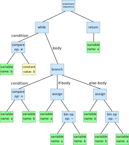
Dcoetzee, CC0, via Wikimedia Commons
As you can see, terminal expressions are constant and variable, non-terminal expressions are the rest.
What is not included
The implementation of the Interpreter does not include parsing the language string input into an AST tree. It is enough to implement classes of terminal, non-terminal expressions, Interpret methods with the Context argument at the input, format the AST tree from expressions, and run the Interpret method at the root expression. The context can be used to store the application state during execution.
Implementation
The pattern involves:
- Client – returns the AST tree and runs Interpret(context) for the root node (Client)
- Context – contains the state of the application, passed to expressions during interpretation (Context)
- Abstract expression – an abstract class containing the Interpret(context) (Expression) method
- A terminal expression is a final expression, a descendant of an abstract expression (TerminalExpression)
- A non-terminal expression is not a final expression, it contains pointers to nodes deep in the AST tree, subordinate nodes usually affect the result of interpreting the non-terminal expression (NonTerminalExpression)
C# Client Example
        static void Main(string[] args)
        {
            var context = new Context();
            var initialProgram = new PerformExpression(
                new IExpression[] {
                    new SetExpression("alpha", "1"),
                    new GetExpression("alpha"),
                    new PrintExpression(
                        new IExpression[] {
                            new ConstantExpression("Hello Interpreter Pattern")
                        }
                    )
                }
            );
            System.Console.WriteLine(initialProgram.interpret(context));
        }
}
Abstract Expression Example in C#
{
    String interpret(Context context);
}
Example of Terminal Expression in C# (String Constant)
{
    private String constant;

    public ConstantExpression(String constant) {
        this.constant = constant;
    }

    override public String interpret(Context context) {
        return constant;
    }
}
Example of Non-Terminal Expression in C# (Start and concatenate results of subordinate nodes, using the separator “;”
{
    public PerformExpression(IExpression[] leafs) : base(leafs) {
        this.leafs = leafs;
    }

    override public String interpret(Context context) {
        var output = "";
        foreach (var leaf in leafs) {
            output += leaf.interpret(context) + ";";
        }
        return output;
    }
}
Can you do it functionally?
As we know, all Turing-complete languages are equivalent. Is it possible to transfer the Object-Oriented pattern to the Functional programming language?
For the experiment, we can take the FP language for the web called Elm. Elm does not have classes, but it does have Records and Types, so the following records and types are involved in the implementation:
- Expression – an enumeration of all possible expressions of the language (Expression)
- Subordinate expression – an expression that is subordinate to a Nonterminal expression (ExpressionLeaf)
- Context – a record that stores the state of the application (Context)
- Functions implementing Interpret(context) methods – all necessary functions implementing the functionality of Terminal, Non-terminal expressions
- Auxiliary records of the Interpreter state – necessary for the correct operation of the Interpreter, store the state of the Interpreter, context
An example of a function implementing interpretation for the entire set of possible expressions in Elm:
  case input.expression of
    Constant text ->
      {
        output = text,
        context = input.context
      }
    Perform leafs ->
      let inputs = List.map (\leaf -> { expressionLeaf = leaf, context = input.context } ) leafs in
        let startLeaf = { expressionLeaf = (Node (Constant "")), context = { variables = Dict.empty } } in
          let outputExpressionInput = List.foldl mergeContextsAndRunLeafs startLeaf inputs in
            {
              output = (runExpressionLeaf outputExpressionInput).output,
              context = input.context
            }
    Print printExpression ->
      run
      {
        expression = printExpression,
        context = input.context
      }
    Set key value ->
      let variables = Dict.insert key value input.context.variables in
      {
        output = "OK",
        context = { variables = variables }
      }
    Get key ->
      {
        output = Maybe.withDefault ("No value for key: " ++ key) (Dict.get key input.context.variables),
        context = input.context
      }
And parse?
Parsing source code into an AST tree is not part of the Interpreter pattern, there are several approaches to parsing source code, but we’ll talk about that some other time.
In the implementation of the Interpreter for Elm, I wrote the simplest parser in the AST tree, consisting of two functions – parsing the node, parsing the subordinate nodes.
parseLeafs state =
    let tokensQueue = state.tokensQueue in
        let popped = pop state.tokensQueue in
            let tokensQueueTail = tail state.tokensQueue in
                if popped == "Nothing" then
                    state
                else if popped == "Perform(" then
                    {
                        tokensQueue = tokensQueue,
                        result = (state.result ++ [Node (parse tokensQueue)])
                    }
                else if popped == ")" then
                    parseLeafs {
                        tokensQueue = tokensQueueTail,
                        result = state.result
                    }
                else if popped == "Set" then
                    let key = pop tokensQueueTail in
                        let value = pop (tail tokensQueueTail) in
                            parseLeafs {
                                tokensQueue = tail (tail tokensQueueTail),
                                result = (state.result ++ [Node (Set key value)])
                            }
                else if popped == "Get" then
                    let key = pop tokensQueueTail in
                        parseLeafs {
                            tokensQueue = tail tokensQueueTail,
                            result = (state.result ++ [Node (Get key)])
                        }
                else
                    parseLeafs {
                        tokensQueue = tokensQueueTail,
                        result = (state.result ++ [Node (Constant popped)])
                    }

parse tokensQueue =
    let popped = pop tokensQueue in
        let tokensQueueTail = tail tokensQueue in
            if popped == "Perform(" then
                Perform (
                    parseLeafs {
                        tokensQueue = tokensQueueTail,
                        result = []
                    }
                ).result
            else if popped == "Set" then
                let key = pop tokensQueueTail in
                    let value = pop (tail tokensQueueTail) in
                        Set key value
            else if popped == "Print" then
                Print (parse tokensQueueTail)
            else
                Constant popped
Links
https://gitlab.com/demensdeum /patterns/-/tree/master/interpreter/elm
https://gitlab.com/demensdeum/patterns/-/tree/master/interpreter/csharp
Sources
https://en.wikipedia.org/wiki/Interpreter_pattern
https://elm-lang.org/
https://docs.microsoft.com/en-us/dotnet/csharp/
RGB image to grayscale
In this note I will describe the algorithm for converting an RGB buffer to grayscale.
And this is done quite simply, each pixel of the buffer’s color channel is transformed according to a certain formula and the output is a gray image.
Average method:
red = average;
green = average;
blue = average;
Складываем 3 цветовых канала и делим на 3.


Однако существует еще один метод – метод средневзвешенный, он учитывает цветовосприятие человека:
red = luminance;
green = luminance;
blue = luminance;

Какой метод лучше использовать? Да какой вам больше подходит для конкретной задачи. Далее сравнение методов с помощью тестовой цветовой сетки:

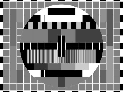
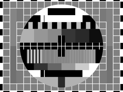
Пример реализации на JavaScript + HTML 5
    image,
    canvas,
    weightedAverage
) {
    const context = canvas.getContext('2d');

    const imageWeight = image.width;
    const imageHeight = image.height;

    canvas.width = imageWeight;
    canvas.height = imageHeight;

    context.drawImage(image, 0, 0);

    let pixels = context
        .getImageData(
            0,
            0,
            imageWeight,
            imageHeight
        );

    for (let y = 0; y & lt; pixels.height; y++) {
        for (let x = 0; x & lt; pixels.width; x++) {
            const i = (y * 4) * pixels.width + x * 4;

            let red = pixels.data[i];
            let green = pixels.data[i + 1];
            let blue = pixels.data[i + 2]

            const average = (red + green + blue) / 3;
            const luminance = 0.2126 * red +
                0.7152 * green +
                0.0722 * blue;

            red = weightedAverage ? luminance : average;
            green = weightedAverage ? luminance : average;
            blue = weightedAverage ? luminance : average;

            pixels.data[i] = red;
            pixels.data[i + 1] = green;
            pixels.data[i + 2] = blue;
        }
    }
    context
        .putImageData(
            pixels,
            0,
            0,
            0,
            0,
            pixels.width,
            pixels.height
        );
}
Источники
https://www.baeldung.com/cs/convert-rgb-to-grayscale
https://twitter.com/mudasobwa/status/1528046455587495940
https://rosettacode.org/wiki/Grayscale_image
Ссылки
http://papugi.demensdeum.repl.co/
Благодарности
Спасибо Aleksei Matiushkin (https://twitter.com/mudasobwa) за наводку на Rosetta Code
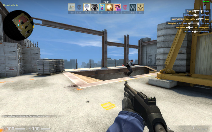
How to Run CSGO on Macbook M1
Turing Computing Machines
I present to your attention a translation of the first pages of Alan Turing’s article “ON COMPUTABLE NUMBERS WITH AN APPLICATION TO THE RESOLUTION PROBLEM” from 1936. The first chapters contain a description of the computing machines that later became the basis for modern computing technology.
The full translation of the article and an explanation can be read in the book by the American popularizer Charles Petzold, entitled “Reading Turing. A Journey Through Turing’s Historic Article on Computability and Turing Machines” (ISBN 978-5-97060-231-7, 978-0-470-22905-7)
Original article:
https://www.astro.puc.cl/~rparra/tools/PAPERS/turing_1936.pdf
—
ON COMPUTABLE NUMBERS WITH AN APPLICATION TO THE DECISION PROBLEM
A. M. TURING
[Received May 28, 1936 – Read November 12, 1936]
“Computable” numbers may be briefly described as real numbers whose expressions as decimal fractions are computable by a finite number of means. Although numbers are at first glance considered computable in this paper, it is almost as easy to define and study computable functions of an integer variable, a real variable, a computable variable, computable predicates, and the like. However, the fundamental problems associated with these computable objects are the same in each case. I have chosen computable numbers as the computable object for our detailed consideration because the methodology for considering them is the least cumbersome. I hope to describe soon the relationships of computable numbers to computable functions, and so forth, involving research in the theory of functions of a real variable expressed in terms of computable numbers. By my definition, a real number is computable if its decimal representation can be written down by a machine.
In sections 9 and 10 I give some arguments to show that computable numbers include all numbers that are naturally considered computable. In particular, I show that some large classes of numbers are computable. These include, for example, the real parts of all algebraic numbers, the real parts of the zeros of the Bessel functions, the numbers π, e, and so on. However, computable numbers do not include all definable numbers, as is demonstrated by an example of a definable number that is not computable.
Although the class of computable numbers is very large and in many ways similar to the class of real numbers, it is still enumerable. In §8 I consider certain arguments that seem to prove the opposite assumption. When one of these arguments is applied correctly, it leads to conclusions that at first glance are similar to those of Gödel.* These results have extremely important applications. In particular, as shown below (§11), the decision problem cannot have a solution.
In a recent paper, Alonzo Church** introduced the idea of ”effective calculability”, which is equivalent to my idea of ”computability” but has a completely different definition. Church also comes to similar conclusions about the resolution problem. A proof of the equivalence of “computability” and “effective calculability” is given in the appendix to this paper.
1. Computing machines
We have already said that computable numbers are those whose decimal places are computable by finite means. A more precise definition is required here. No real attempt will be made in this paper to justify the definitions given here until we reach §9. For now I will merely note that the (logical) justification (for this) is that human memory is necessarily limited.
Let us compare a man in the process of calculating a real number with a machine that is capable of fulfilling only a finite number of conditions q1, q2, …, qR; let us call these conditions “m-configurations”. The given (i.e. so defined) machine is equipped with a “tape” (analogous to paper). Such a tape, passing through the machine, is divided into sections. Let us call them “squares”. Each such square can contain some “symbol”. At any moment there exists and, moreover, only one such square, say, the r-th, containing the symbol that is “in the given machine”. Let us call such a square a “scanned symbol”. A “scanned symbol” is the only such symbol of which the machine, figuratively speaking, is “directly aware”. However, when changing its m-configuration, the machine can effectively remember some symbols that it “saw” (scanned) earlier. The possible behavior of the machine at any moment is determined by the m-configuration qn and the scanned symbol***. Let us call this pair of symbols qn, a “configuration”. A configuration so designated determines the possible behavior of the machine. In some of these configurations, in which the scanned square is empty (i.e., does not contain a symbol), the machine writes a new symbol on the scanned square, and in other of these configurations it erases the scanned symbol. The machine can also move on to scanning another square, but in this case it can only move to the adjacent square to the right or left. In addition to any of these operations, the m-configuration of the machine can be changed. In this case, some of the written symbols will form a sequence of digits that is the decimal part of the real number being calculated. The rest will be no more than fuzzy marks to “help the memory”. In this case, only the fuzzy marks mentioned above can be erased.
I claim that the operations considered here include all those used in computing. The reason for this claim is easier to understand for a reader with some understanding of machine theory. Therefore, in the next section I will continue to develop the theory under consideration, relying on an understanding of the meaning of the terms “machine”, “tape”, “scanned”, etc.
*Goedel, “On the Formally Undecidable Propositions of the Principles of Mathematics (published by Whitehead and Russell in 1910, 1912 and 1913) and Related Systems, Part I,” Journal of Mathematical Physics, Monthly Bulletin in German, No. 38 (for 1931, pp. 173-198).
** Alonzo Church, “An Unsolvable Problem in Elementary Number Theory,” American J. of Math., no. 58 (1936), pp. 345-363.
*** Alonzo Church, “A Note on the Resolution Problem,” J. of Symbolic Logic, no. 1 (1936), pp. 40-41
Turing Bomb
In 1936, scientist Alan Turing in his publication “On Computable Numbers, With An Application to Entscheidungsproblem” describes the use of a universal computing machine that could put an end to the question of the solvability problem in mathematics. As a result, he comes to the conclusion that such a machine would not be able to solve anything correctly if the result of its work was inverted and looped back to itself. It turns out that it is impossible to create an *ideal* antivirus, an *ideal* tile layer, a program that suggests ideal phrases for your crash, etc. Paradox!
However, this universal computing machine can be used to implement any algorithm, which is what British intelligence took advantage of by hiring Turing and allowing him to create the “Bombe” machine to decipher German messages during World War II.
The following is an OOP simulation of a single-tape computer in Dart, based on the original document.
A Turing machine consists of a film divided into sections, each section contains a symbol, the symbols can be read or written. An example of a film class:
final _map = Map<int, String>();

  String read({required int at}) {
    return _map[at] ?? "";
  }

  void write({required String symbol, required int at}) {
    _map[at] = symbol;
  }
}
There is also a “scanning square”, it can move along the film, read or write information, in modern language – a magnetic head. An example of a magnetic head class:
  int _index = 0;
  InfiniteTape _infiniteTape;
  TapeHead(this._infiniteTape) {}

  String next() {
    _index += 1;
    move(to: _index);
    final output = read();
    return output;
  }

  String previous() {
    _index -= 1;
    move(to: _index);
    final output = read();
    return output;
  }

  void move({required int to}) {
    this._index = to;
  }

  String read() {
    return _infiniteTape.read(at: this._index);
  }

  void write(String symbol) {
    _infiniteTape.write(symbol: symbol, at: this._index);
  }

  int index() {
    return _index;
  }
}
The machine contains “m-configurations” by which it can decide what to do next. In modern language, these are states and state handlers. An example of a state handler:
  FiniteStateControlDelegate? delegate = null;

  void handle({required String symbol}) {
    if (symbol == OPCODE_PRINT) {
      final argument = delegate?.nextSymbol();
      print(argument);
    }
    else if (symbol == OPCODE_GENERATE_RANDOM_NUMBER_FROM_ZERO_TO_AND_WRITE_AFTER) {
      final to = int.tryParse(delegate!.nextSymbol())!;
      final value = new Random().nextInt(to);
      delegate!.nextSymbol();
      delegate!.write(value.toString());
    }
    else if (symbol == OPCODE_INPUT_TO_NEXT) {
      final input = stdin.readLineSync()!;
      delegate?.nextSymbol();
      delegate?.write(input);
    }
    else if (symbol == OPCODE_COPY_FROM_TO) {
      final currentIndex = delegate!.index();

и т.д.
After this, you need to create “configurations”, in modern language these are operation codes (opcodes), their handlers. An example of opcodes:
const OPCODE_PRINT = "print";
const OPCODE_INCREMENT_NEXT = "increment next";
const OPCODE_DECREMENT_NEXT = "decrement next";
const OPCODE_IF_PREVIOUS_NOT_EQUAL = "if previous not equal";
const OPCODE_MOVE_TO_INDEX = "move to index";
const OPCODE_COPY_FROM_TO = "copy from index to index";
const OPCODE_INPUT_TO_NEXT = "input to next";
const OPCODE_GENERATE_RANDOM_NUMBER_FROM_ZERO_TO_AND_WRITE_AFTER = "generate random number from zero to next and write after";
Don’t forget to create an opcode and a stop handler, otherwise you won’t be able to prove or not prove (sic!) the resolution problem.
Now, using the “mediator” pattern, we connect all the classes in the Turing Machine class, create an instance of the class, record the programs on tape using a tape recorder, load the tape and you can use it!
For me personally, the question of what came first remains interesting: the creation of a universal computer or the proof of the “Entscheidungsproblem”, which resulted in the computer appearing as a by-product.
Cassettes
For fun, I recorded several cassette programs for my version of the machine.
Hello World
hello world
stop
Считаем до 16-ти
0
if previous not equal
16
copy from index to index
1
8
print
?
move to index
0
else
copy from index to index
1
16
print
?
print
Finished!
stop
Самой интересной задачей было написание Quine программы, которая печатает свой исходный код, для одноленточной машины. Первые 8 часов мне казалось что эта задача не решаема с таким малым количеством опкодов, однако всего через 16 часов оказалось что я был не прав.
Реализация и примеры кассет, источники ниже.
Ссылки
https://gitlab.com/demensdeum/turing-machine
Источники
https://www.astro.puc.cl/~rparra/tools/PAPERS/turing_1936.pdf
https://kpolyakov.spb.ru/prog/turing.htm
https://www.youtube.com/watch?v=dNRDvLACg5Q
https://www.youtube.com/watch?v=jP3ceURvIYc
https://www.youtube.com/watch?v=9QCJj5QzETI
https://www.youtube.com/watch?v=HeQX2HjkcNo&t=0s
Writing Assembler for Sega Genesis #5
In this post I will describe the process of reading the joystick, changing the sprite position, horizontal flip, Sega Genesis emulator and potentially the console itself.
Reading of presses, processing of “events” of the Sega joystick occurs according to the following scheme:
- Request for combination of bits of pressed buttons
- Reading bits of pressed buttons
- Processing at the game logic level
To move the skeleton sprite we need to store the current position variables.
RAM
Game logic variables are stored in RAM, people haven’t come up with anything better yet. Let’s declare variable addresses, change the rendering code:
skeletonYpos = $FF0002
frameCounter = $FF0004
skeletonHorizontalFlip = $FF0006

    move.w #$0100,skeletonXpos
    move.w #$0100,skeletonYpos
    move.w #$0001,skeletonHorizontalFlip

FillSpriteTable:
    move.l #$70000003,vdp_control_port
    move.w skeletonYpos,vdp_data_port
    move.w #$0F00,vdp_data_port
    move.w skeletonHorizontalFlip,vdp_data_port
    move.w skeletonXpos,vdp_data_port
As you can see, the address available for work starts at 0xFF0000 and ends at 0xFFFFFF, so we have 64 KB of memory available. Skeleton positions are declared at skeletonXpos, skeletonYpos, horizontal flip at skeletonHorizontalFlip.
Joypad
Similar to VDP, joypads are handled via two separate ports – the control port and the data port, for the first one it’s 0xA10009 and 0xA10003 respectively. When working with a joypad, there’s one interesting feature – first you need to request a combination of buttons for polling, and then, after waiting for the bus update, read the required presses. For the C/B buttons and the cross, it’s 0x40, an example below:
  move.b #$40,joypad_one_control_port; C/B/Dpad
  nop ; bus sync
  nop ; bus sync
  move.b joypad_one_data_port,d2
  rts
The state of the buttons pressed or not pressed will remain in the d2 register, in general, what was requested via the data port will remain. After that, go to the Motorola 68000 register viewer of your favorite emulator, see what the d2 register is equal to depending on the presses. You can find this out in the manual in a smart way, but we don’t take your word for it. Next, processing the pressed buttons in the d2 register
    cmp #$FFFFFF7B,d2; handle left
    beq MoveLeft
    cmp #$FFFFFF77,d2; handle right
    beq MoveRight
    cmp #$FFFFFF7E,d2; handle up
    beq MoveUp
    cmp #$FFFFFF7D,d2; handle down
    beq MoveDown
    rts
Проверять нужно конечно отдельные биты, а не целыми словами, но пока и так сойдет. Теперь осталось самое простое – написать обработчики всех событий перемещения по 4-м направлениям. Для этого меняем переменные в RAM, и запускаем процедуру перерисовки.
Пример для перемещения влево + изменение горизонтального флипа:
    move.w skeletonXpos,d0
    sub.w #1,d0
    move.w d0,skeletonXpos
    move.w #$0801,skeletonHorizontalFlip
    jmp FillSpriteTable
После добавления всех обработчиков и сборки, вы увидите как скелет перемещается и поворачивается по экрану, но слишком быстро, быстрее самого ежа Соника.
Не так быстро!
Чтобы замедлить скорость игрового цикла, существуют несколько техник, я выбрал самую простую и не затрагивающую работу с внешними портами – подсчет цифры через регистр пока она не станет равна нулю.
Пример замедляющего цикла и игрового цикла:
  move.w #512,frameCounter
WaitFrame:
  move.w frameCounter,d0
  sub.w #1,d0
  move.w d0,frameCounter
  dbra d0,WaitFrame
GameLoop:
  jsr ReadJoypad
  jsr HandleJoypad
  jmp GameLoop
After that, the skeleton runs slower, which is what was required. As far as I know, the most common option for “slowing down” is counting the vertical sync flag, you can count how many times the screen was drawn, thus tying it to a specific fps.
Links
https://gitlab .com/demensdeum/segagenesisamples/-/blob/main/8Joypad/vasm/main.asm
Sources
https://www.chibiakumas.com/68000/platform2.php
https://huguesjohnson.com/programming/genesis/tiles-sprites/
Writing Assembler for Sega Genesis #4
In this note I will describe how to draw sprites using the VDP emulator of the Sega Genesis console.
The process of rendering sprites is very similar to rendering tiles:
- Loading colors into CRAM
- Unloading 8×8 sprite parts into VRAM
- Filling Sprite Table in VRAM
For example, let’s take a sprite of a skeleton with a sword 32×32 pixels
Skeleton Guy [Animated] by Disthorn
CRAM
Using ImaGenesis we will convert it into CRAM colors and VRAM patterns for assembler. After that we will get two files in asm format, then we will rewrite the colors to word size, and the tiles should be put in the correct order for drawing.
Interesting information: you can switch the VDP autoincrement via register 0xF to the word size, this will allow you to remove the address increment from the CRAM color fill code.
VRAM
The Sega manual has the correct tile order for large sprites, but we’re smarter, so we’ll take the indexes from the ChibiAkumas blog, starting the count from index 0:
0 4 8 12
1 5 9 13
2 6 10 14
3 7 11 15
Why is everything upside down? What do you expect, the prefix is Japanese! It could have been from right to left!
Let’s change the order manually in the sprite asm file:
	dc.l	$11111111	; Tile #0
	dc.l	$11111111
	dc.l	$11111111
	dc.l	$11111111
	dc.l	$11111111
	dc.l	$11111111
	dc.l	$11111111
	dc.l	$11111111
	dc.l	$11111111	; Tile #4
	dc.l	$11111111
	dc.l	$11111111
	dc.l	$11111111
	dc.l	$11111111
	dc.l	$11111111
	dc.l	$11111111
	dc.l	$11111111
	dc.l	$11111111	; Tile #8
	dc.l	$11111111
	dc.l	$11111111
	dc.l	$11111111
	dc.l	$11111111
	dc.l	$11111122
	dc.l	$11111122
	dc.l	$11111166
	dc.l	$11111166	; Tile #12
	dc.l	$11111166
	dc.l	$11111166
	и т.д.
Load the sprite like regular tiles/patterns:
  lea Sprite,a0
  move.l #$40200000,vdp_control_port; write to VRAM command
  move.w #128,d0 ; (16*8 rows of sprite) counter
SpriteVRAMLoop:
  move.l (a0)+,vdp_data_port;
  dbra d0,SpriteVRAMLoop
To draw the sprite, it remains to fill the sprite table (Sprite Table)
Sprite Table
The sprite table is filled in VRAM, its location address is set in VDP register 0x05, the address is again tricky, you can look it up in the manual, an example for address F000:
Ок, теперь запишем наш спрайт в таблицу. Для этого нужно заполнить “структуру” данных состоящую из четырех word. Бинарное описание структуры вы можете найти в мануале. Лично я сделал проще, таблицу спрайтов можно редактировать вручную в эмуляторе Exodus.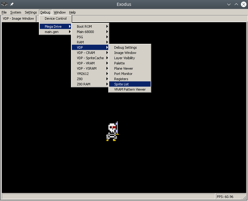
The parameters of the structure are obvious from the name, for example XPos, YPos – coordinates, Tiles – the number of the starting tile for drawing, HSize, VSize – the size of the sprite by adding parts 8×8, HFlip, VFlip – hardware rotations of the sprite horizontally and vertically.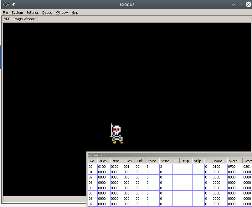
It is very important to remember that sprites can be off-screen, this is correct behavior, since unloading off-screen sprites from memory is quite a resource-intensive task.
After filling the data in the emulator, it needs to be copied from VRAM to address 0xF000, Exodus also supports this feature.
By analogy with drawing tiles, first we access the VDP control port to start writing at address 0xF000, then we write the structure to the data port.
Let me remind you that the description of VRAM addressing can be read in the manual or in the blog Nameless Algorithm.
In short, VDP addressing works like this:
[..DC BA98 7654 3210 …. …. …. ..FE]
Where hex is the bit position in the desired address. The first two bits are the type of command requested, for example 01 – write to VRAM. Then for address 0XF000 you get:
0111 0000 0000 0000 0000 0000 0000 0011 (70000003)
As a result we get the code:
  move.l #$70000003,vdp_control_port
  move.w #$0100,vdp_data_port
  move.w #$0F00,vdp_data_port
  move.w #$0001,vdp_data_port
  move.w #$0100,vdp_data_port
After this, the skeleton sprite will be displayed at coordinates 256, 256. Cool, huh?
Links
https://gitlab.com/demensdeum /segagenesissamples/-/tree/main/7Sprite/vasm
https://opengameart.org/content/skeleton-guy-animated
Sources
https://namelessalgorithm.com/genesis/blog/vdp/
https://www.chibiakumas.com/68000/platform3.php#LessonP27
https://plutiedev.com/sprites
Writing Assembler for Sega Genesis #3
In this note I will describe how to display an image from tiles on the Sega Genesis emulator using assembler.
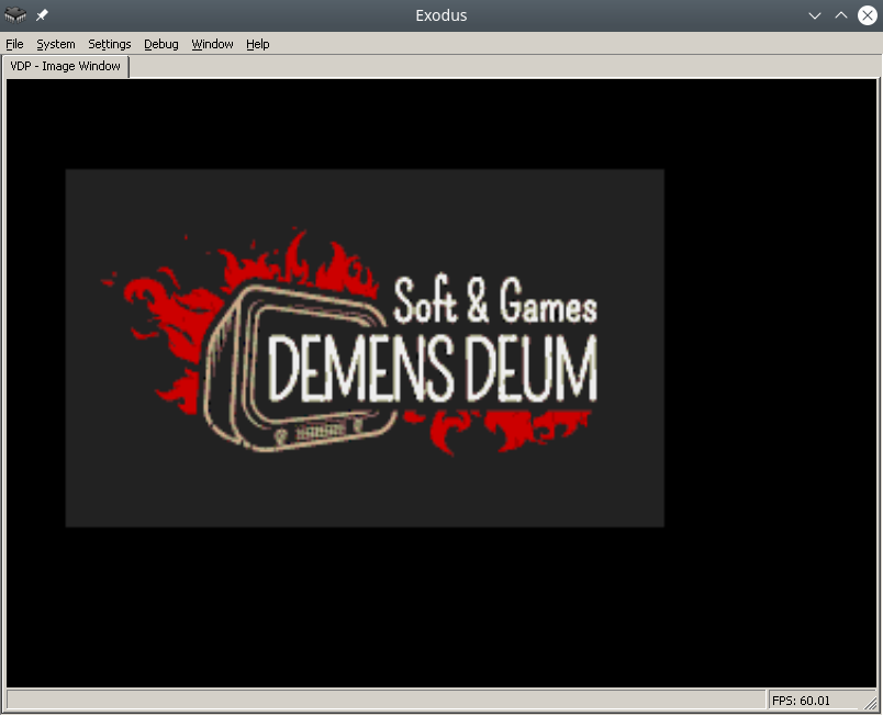
The splash image Demens Deum in the Exodus emulator will look like this:
The process of outputting a PNG image using tiles is done step by step:
- Reduce image to fit Sega screen
- Convert PNG to assembly data code, with separation into colors and tiles
- Loading color palette into CRAM
- Loading tiles/patterns into VRAM
- Loading tile indices to Plane A/B addresses into VRAM
- You can reduce the image to the size of the Sega screen using your favorite graphics editor, such as Blender.
PNG conversion
To convert images, you can use the ImaGenesis tool, to work under wine, you need Visual Basic 6 libraries, they can be installed using winetricks (winetricks vb6run), or RICHTX32.OCX can be downloaded from the Internet and placed in the application folder for correct operation.
In ImaGenesis, you need to select 4-bit color, export colors and tiles to two assembler files. Then, in the file with colors, you need to put each color into a word (2 bytes), for this, the opcode dc.w is used.
For example CRAM splash screen:
  dc.w $0000
  dc.w $0000
  dc.w $0222
  dc.w $000A
  dc.w $0226
  dc.w $000C
  dc.w $0220
  dc.w $08AA
  dc.w $0446
  dc.w $0EEE
  dc.w $0244
  dc.w $0668
  dc.w $0688
  dc.w $08AC
  dc.w $0200
  dc.w $0000
Leave the tile file as is, it already contains the correct format for loading. Example of part of the tile file:
	dc.l	$11111111	; Tile #0
	dc.l	$11111111
	dc.l	$11111111
	dc.l	$11111111
	dc.l	$11111111
	dc.l	$11111111
	dc.l	$11111111
	dc.l	$11111111
	dc.l	$11111111	; Tile #1
	dc.l	$11111111
	dc.l	$11111111
	dc.l	$11111111
	dc.l	$11111111
	dc.l	$11111111
	dc.l	$11111111
	dc.l	$11111111
As you can see from the example above, the tiles are an 8×8 grid of CRAM color palette indices.
Colors in CRAM
Loading into CRAM is done by setting the color load command at a specific CRAM address in the control port (vdp control). The command format is described in the Sega Genesis Software Manual (1989), I will only add that it is enough to add 0x20000 to the address to move to the next color.
Next, you need to load the color into the data port (vdp data); The easiest way to understand the loading is with the example below:
    lea Colors,a0 ; pointer to Colors label
    move.l #15,d7; colors counter
VDPCRAMFillLoopStep:
    move.l  d0,vdp_control_port ;
    move.w  (a0)+,d1;
    move.w  d1,(vdp_data_port);
    add.l #$20000,d0 ; increment CRAM address
    dbra d7,VDPCRAMFillLoopStep
Tiles in VRAM
Next comes loading of tiles/patterns into the VRAM video memory. To do this, select an address in VRAM, for example 0x00000000. By analogy with CRAM, we address the VDP control port with a command to write to VRAM and the starting address.
After that, you can upload longwords to VRAM, compared to CRAM, you do not need to specify the address for each longword, since there is a VRAM autoincrement mode. You can enable it using the VDP register flag 0x0F (dc.b $02)
  lea Tiles,a0
  move.l #$40200000,vdp_control_port; write to VRAM command
  move.w #6136,d0 ; (767 tiles * 8 rows) counter
TilesVRAMLoop:
  move.l (a0)+,vdp_data_port;
  dbra d0,TilesVRAMLoop
Tile indexes in Plane A/B
Now we need to fill the screen with tiles by their index. To do this, fill the VRAM at the address Plane A/B, which is set in the VDP registers (0x02, 0x04). More details about the tricky addressing are in the Sega manual, in my example the VRAM address is 0xC000, we will unload the indices there.
Your image will fill the off-screen VRAM space anyway, so after drawing the screen space, your renderer should stop drawing and continue again when the cursor moves to a new line. There are many options for how to implement this, I used the simplest option of counting on two registers of the image width counter, the cursor position counter.
Code example:
  move.w #0,d0     ; column index
  move.w #1,d1     ; tile index
  move.l #$40000003,(vdp_control_port) ; initial drawing location
  move.l #2500,d7     ; how many tiles to draw (entire screen ~2500)

imageWidth = 31
screenWidth = 64

FillBackgroundStep:
  cmp.w	#imageWidth,d0
  ble.w	FillBackgroundStepFill
FillBackgroundStep2:
  cmp.w	#imageWidth,d0
  bgt.w	FillBackgroundStepSkip
FillBackgroundStep3:
  add #1,d0
  cmp.w	#screenWidth,d0
  bge.w	FillBackgroundStepNewRow
FillBackgroundStep4:
  dbra d7,FillBackgroundStep    ; loop to next tile

Stuck:
  nop
  jmp Stuck

FillBackgroundStepNewRow:
  move.w #0,d0
  jmp FillBackgroundStep4
FillBackgroundStepFill:
  move.w d1,(vdp_data_port)    ; copy the pattern to VPD
  add #1,d1
  jmp FillBackgroundStep2
FillBackgroundStepSkip:
  move.w #0,(vdp_data_port)    ; copy the pattern to VPD
  jmp FillBackgroundStep3
After that, all that remains is to compile the ROM using vasm, run the simulator, and see the picture.
Debugging
Not everything will work out right away, so I want to recommend the following Exodus emulator tools:
- m68k processor debugger
- Changing the number of m68k processor cycles (for slow-mo mode in the debugger)
- Viewers CRAM, VRAM, Plane A/B
- Carefully read the documentation for m68k, the opcodes used (not everything is as obvious as it seems at first glance)
- View code/disassembly examples of games on github
- Implement subroutines of processor exceptions, handle them
Pointers to subroutines of processor exceptions are placed in the ROM header, also on GitHub there is a project with an interactive runtime debugger for Sega, called genesis-debugger.
Use all the tools available, have fun old school coding and may Blast Processing be with you!
Links
https://gitlab.com/demensdeum /segagenesisamples/-/tree/main/6Image/vasm
http://devster.monkeeh.com/sega/imagenesis/
https://github.com/flamewing/genesis-debugger
Sources
https://www.chibiakumas.com/68000/helloworld .php#LessonH5
https://huguesjohnson.com/programming/genesis/tiles-sprites/
Writing Assembler for Sega Genesis #2
In this note I will describe how to load colors into the Sega palette in assembler.
The final result in the Exodus emulator will look like this: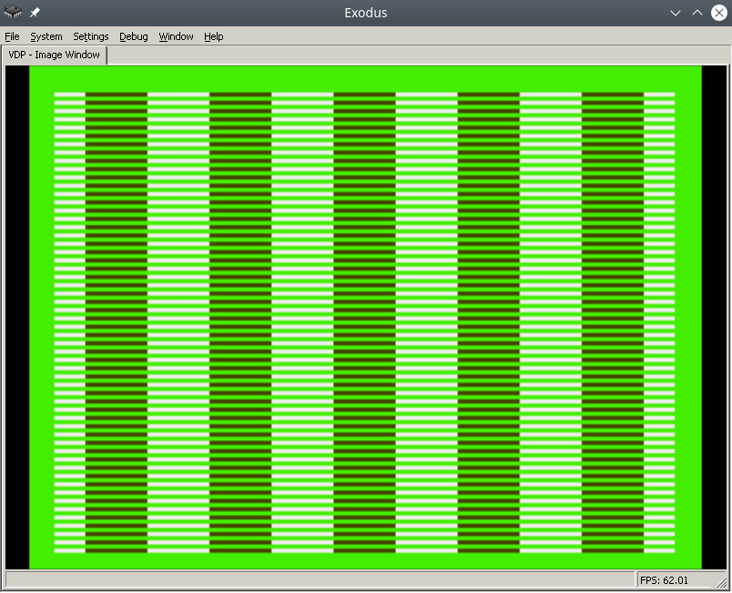
To make the process easier, find a pdf online called Genesis Software Manual (1989), it describes the whole process in great detail, in fact, this note is a commentary on the original manual.
In order to write colors to the VDP chip of the Sega emulator, you need to do the following:
- Disable TMSS protection system
- Write the correct parameters to the VDP registers
- Write the desired colors to CRAM
For assembly we will use vasmm68k_mot and a favorite text editor, for example echo. Assembly is carried out by the command:
Порты VDP
VDP чип общается с M68K через два порта в оперативной памяти – порт контроля и порт данных.
По сути:
- Через порт контроля можно выставлять значения регистрам VDP.
- Также порт контроля является указателем на ту часть VDP (VRAM, CRAM, VSRAM etc.) через которую передаются данные через порт данных
Интересная информация: Сега сохранила совместимость с играми Master System, на что указывает MODE 4 из мануала разработчика, в нем VDP переключается в режим Master System.
Объявим порты контроля и данных:
vdp_data_port = $C00000
Отключить систему защиты TMSS
Защита от нелицензионных игр TMSS имеет несколько вариантов разблокировки, например требуется чтобы до обращения к VDP в адресном регистре A1 лежала строка “SEGA”.
MOVE.B A1,D0; Получаем версию хардвары цифрой из A1 в регистр D0
ANDI.B 0x0F,D0; По маске берем последние биты, чтобы ничего не сломать
BEQ.B SkipTmss; Если версия равна 0, скорее всего это японка или эмулятор без включенного TMSS, тогда идем в сабрутину SkipTmss
MOVE.L "SEGA",A1; Или записываем строку SEGA в A1
Write the correct parameters to the VDP registers
Why set the correct parameters in the VDP registers at all? The idea is that the VDP can do a lot, so before drawing you need to initialize it with the necessary features, otherwise it simply won't understand what you want from it.
Each register is responsible for a specific setting/operating mode. The Sega manual specifies all the bits/flags for each of the 24 registers, and a description of the registers themselves.
Let's take ready-made parameters with comments from the bigevilcorporation blog:
VDPReg0: dc.b $14 ; 0: H interrupt on, palettes on
VDPReg1: dc.b $74 ; 1: V interrupt on, display on, DMA on, Genesis mode on
VDPReg2: dc.b $30 ; 2: Pattern table for Scroll Plane A at VRAM $C000
; (bits 3-5 = bits 13-15)
VDPReg3: dc.b $00 ; 3: Pattern table for Window Plane at VRAM $0000
; (disabled) (bits 1-5 = bits 11-15)
VDPReg4: dc.b $07 ; 4: Pattern table for Scroll Plane B at VRAM $E000
; (bits 0-2 = bits 11-15)
VDPReg5: dc.b $78 ; 5: Sprite table at VRAM $F000 (bits 0-6 = bits 9-15)
VDPReg6: dc.b $00 ; 6: Unused
VDPReg7: dc.b $00 ; 7: Background colour - bits 0-3 = colour,
; bits 4-5 = palette
VDPReg8: dc.b $00 ; 8: Unused
VDPReg9: dc.b $00 ; 9: Unused
VDPRegA: dc.b $FF ; 10: Frequency of Horiz. interrupt in Rasters
; (number of lines travelled by the beam)
VDPRegB: dc.b $00 ; 11: External interrupts off, V scroll fullscreen,
; H scroll fullscreen
VDPRegC: dc.b $81 ; 12: Shadows and highlights off, interlace off,
; H40 mode (320 x 224 screen res)
VDPRegD: dc.b $3F ; 13: Horiz. scroll table at VRAM $FC00 (bits 0-5)
VDPRegE: dc.b $00 ; 14: Unused
VDPRegF: dc.b $02 ; 15: Autoincrement 2 bytes
VDPReg10: dc.b $01 ; 16: Vert. scroll 32, Horiz. scroll 64
VDPReg11: dc.b $00 ; 17: Window Plane X pos 0 left
; (pos in bits 0-4, left/right in bit 7)
VDPReg12: dc.b $00 ; 18: Window Plane Y pos 0 up
; (pos in bits 0-4, up/down in bit 7)
VDPReg13: dc.b $FF ; 19: DMA length lo byte
VDPReg14: dc.b $FF ; 20: DMA length hi byte
VDPReg15: dc.b $00 ; 21: DMA source address lo byte
VDPReg16: dc.b $00 ; 22: DMA source address mid byte
VDPReg17: dc.b $80 ; 23: DMA source address hi byte,
; memory-to-VRAM mode (bits 6-7)
Okay, now let's go to the control port and write all the flags to the VDP registers:
move.l #VDPRegisters,a0 ; Пишем адрес таблицы параметров в A1
move.l #$18,d0 ; Счетчик цикла - 24 = 18 (HEX) в D0
move.l #$00008000,d1 ; Готовим команду на запись в регистр VDP по индексу 0, по мануалу - 1000 0000 0000 0000 (BIN) = 8000 (HEX)
FillInitialStateForVDPRegistersLoop:
move.b (a0)+,d1 ; Записываем в D1 итоговое значение регистра VDP из таблицы параметров, на отправку в порт контроля VDP
move.w d1,vdp_control_port ; Отправляем итоговую команду + значение из D1 в порт контроля VDP
add.w #$0100,d1 ; Поднимаем индекс регистра VDP на 1 (бинарное сложение +1 к индексу по мануалу Сеги)
dbra d0,FillInitialStateForVDPRegistersLoop ; Уменьшаем счетчик регистров, продолжаем цикл если необходимо
Самое сложное это прочитать мануал и понять в каком формате подаются данные на порт контроля, опытные разработчики разберутся сразу, а вот неопытные… Немного подумают и поймут, что синтаксис для записи регистров такой:
0B100(5 бит – индекс регистра)(8 бит/байт – значение)
0B1000001001000101 – записать в регистр VDP 2 (00010), значение флажков 01000101.
Записать нужные цвета в CRAM
Далее идем писать два цвета в память цветов CRAM (Color RAM). Для этого пишем в порт контроля команду на доступ к цвету по индексу 0 в CRAM и отправляем по дата порту цвет. Все!
Пример:
move.l #$C0000000,vdp_control_port ; Доступ к цвету по индексу 0 в CRAM через порт контроля
move.w #228,d0; Цвет в D0
move.w d0,vdp_data_port; Отправляем цвет в порт данных
After building and running in the emulator in Exodus, you should have a screen filled with color 228.
Let's fill it with a second color, at the last byte 127.
move.l #$C07f0000,vdp_control_port ; Доступ к цвету по байту 127 в CRAM через порт контроля
move.w #69,d0; Цвет в D0
move.w d0,vdp_data_port; Отправляем цвет в порт данных
Links
https://gitlab.com/demensdeum/segagenesissamples
https://www.exodusemulator.com/
http://sun.hasenbraten.de/vasm/
https://tomeko.net/online_tools/bin_to_32bit_hex.php?lang=en
Sources
https://namelessalgorithm.com/genesis/blog/genesis/
https://plutiedev.com/vdp-commands
https://huguesjohnson.com/programming/genesis/palettes/
https://www.chibiakumas.com/68000/helloworld.php#LessonH5
https://blog.bigevilcorporation.co.uk/2012/03/09/sega-megadrive-3-awaking-the-beast/
Writing Assembler for Sega Genesis #1
The first article dedicated to writing games for the classic Sega Genesis console in Motorola 68000 Assembler.
Let’s write the simplest infinite loop for Sega. For this we will need: assembler, emulator with disassembler, favorite text editor, basic understanding of Sega ROM structure.
For development, I use my own assembler/Dizassembler GEN68KRYBABY:
https://gitlab.com/demensdeum/gen68krybaby/
The tool is developed in Python 3, for assembly a file with the extension .asm or .gen68KryBabyDisasm is fed to the input, the output is a file with the extension .gen68KryBabyAsm.bin, which can be run in an emulator or on a real console (be careful, move away, the console may explode!)
ROM disassembly is also supported, for this you need to supply a ROM file to the input, without the .asm or .gen68KryBabyDisasm extensions. Opcode support will increase or decrease depending on my interest in the topic, the participation of contributors.
Structure
The Sega ROM header takes up the first 512 bytes. It contains information about the game, the title, supported peripherals, checksum, and other system flags. I assume that without the header, the console won’t even look at the ROM, thinking that it’s invalid, like “what are you giving me here?”
After the header comes the Reset subroutine/subprogram, with it the m68K processor starts working. Okay, now it’s a small matter – find the opcodes (operation codes), namely, doing nothing(!) and jumping to the subroutine at the address in memory. Googling, you can find the NOP opcode, which does nothing, and the JSR opcode, which performs an unconditional jump to the argument address, that is, it simply moves the carriage where we ask it to, without any whims.
Putting it all together
The title donor for the ROM was one of the games in the Beta version, currently written as hex data.
00 ff 2b 52 00 00 02 00 00 00 49 90 00 00 49 90 00 00 49 90 00...и т.д.
Код программы со-но представляет из себя объявление сабрутины Reset/EntryPoint в 512 (0x200) байте, NOP, возврат каретки к 0x00000200, таким образом мы получим бесконечный цикл.
Ассемблерный код сабрутины Reset/EntryPoint:
NOP
NOP
NOP
NOP
NOP
JSR 0x00000200
Full example with rom title:
https://gitlab.com /demensdeum/segagenesisamples/-/blob/main/1InfiniteLoop/1infiniteloop.asm
Next we collect:
Запускаем ром 1infiniteloop.asm.gen68KryBabyAsm.bin в режиме дебаггера эмулятора Exodus/Gens, смотрим что m68K корректно считывает NOP, и бесконечно прыгает к EntryPoint в 0x200 на JSR
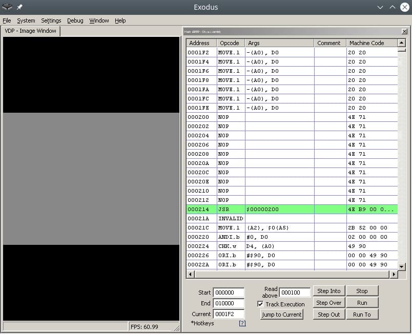
Здесь должен быть Соник показывающий V, но он уехал на Вакен.
Ссылки
https://gitlab.com/demensdeum/gen68krybaby/
https://gitlab.com/demensdeum/segagenesissamples
https://www.exodusemulator.com/downloads/release-archive
Источники
ROM Hacking Demo – Genesis and SNES games in 480i
https://www.chibiakumas.com/68000/genesis.php
https://plutiedev.com/rom-header
https://blog.bigevilcorporation.co.uk/2012/02/28/sega-megadrive-1-getting-started/
https://opensource.apple.com/source/cctools/cctools-836/as/m68k-opcode.h.auto.html
How I didn’t hit the guy on the pole or a story about amazing ingenuity
In this note I will write about the importance of architectural decisions in the development, support of the application, in the conditions of team development.
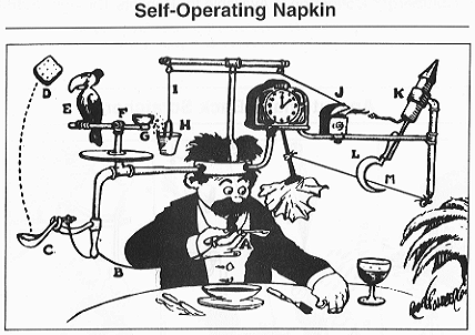
Professor Lucifer Gorgonzola’s Self-Operating Napkin. Rube Goldberg
In my youth, I worked on an app for ordering a taxi. In the program, you could choose a pickup point, a drop point, calculate the cost of the trip, the type of tariff, and, in fact, order a taxi. I got the application at the last stage of pre-launch, after adding several fixes, the application was released in the AppStore. Already at that stage, the whole team understood that it was implemented very poorly, design patterns were not used, all components of the system were tightly connected, in general, it could have been written into one large solid class (God object), nothing would have changed, since the classes mixed their boundaries of responsibility and, in general, overlapped each other with a dead link. Later, the management decided to write the application from scratch, using the correct architecture, which was done and the final product was implemented to several dozen B2B clients.
However, I will describe a funny incident from the previous architecture, from which I sometimes wake up in a cold sweat in the middle of the night, or suddenly remember in the middle of the day and start laughing hysterically. The thing is that I couldn’t hit the guy on the pole the first time, and this brought down most of the application, but first things first.
It was a normal working day, one of the customers gave me a task to slightly improve the design of the application – just move the icon in the center of the pickup address selection screen up a few pixels. Well, having professionally estimated the task at 10 minutes, I moved the icon up 20 pixels, completely unsuspecting, I decided to check the taxi order.
What? The app doesn’t show the order button anymore? How did that happen?
I couldn’t believe my eyes, after raising the icon by 20 pixels the app stopped showing the continue order button. After reverting the change I saw the button again. Something was wrong here. After sitting in the debugger for 20 minutes I got a little tired of unwinding the spaghetti of overlapping class calls, but I found that *moving the image really changes the logic of the app*
The whole thing was in the icon in the center – a man on a pole, when the map was moved, he jumped up to animate the camera movement, this animation was followed by the disappearance of the button at the bottom. Apparently, the program thought that the man, moved by 20 pixels, was jumping, so according to internal logic, it hid the confirmation button.
How can this happen? Does the *state* of the screen depend not on the pattern of the state machine, but on the *representation* of the position of the man on the pole?
That’s exactly what happened, every time the map was drawn, the application *visually poked* the middle of the screen and checked what was there, if there was a guy on a pole, it meant that the map shift animation had ended and the button needed to be shown. If there was no guy there, it meant that the map was shifting and the button needed to be hidden.
Everything is great in the example above, firstly it is an example of a Goldberg Machine (smart machines), secondly it is an example of a developer’s unwillingness to somehow interact with other developers in the team (try to figure it out without me), thirdly you can list all the problems with SOLID, patterns (code smells), violation of MVC and much, much more.
Try not to do this, develop in all possible directions, help your colleagues in their work. Happy New Year to all)
Links
https://ru.wikipedia.org/wiki/Goldberg_Machine
https://ru.wikipedia.org/wiki/SOLID
https://refactoring.guru/ru/refactoring/smells
https://ru.wikipedia.org/wiki/Model -View-Controller
https://refactoring.guru/ru/design-patterns/state
Guess the group
In this note I will describe working with the fasttext text classifier.
Fasttext is a machine learning library for text classification. Let’s try to teach it to identify a metal band by the title of a song. To do this, we will use supervised learning using a dataset.
Let’s create a dataset of songs with band names:
__label__metallica fuel
__label__metallica escape
__label__black_sabbath gypsy
__label__black_sabbath snowblind
__label__black_sabbath am i going insane
__label__anthrax anthrax
__label__anthrax i'm alive
__label__anthrax antisocial
[и т.д.]
Формат обучающей выборки:
Обучим fasttext и сохраним модель:
model.save_model("model.bin")
Let's load the trained model and ask it to identify the band by the song title:
predictResult = model.predict("Bleed")
print(predictResult)
В результате мы получим список классов на которые похож данный пример, с указанием уровня похожести цифрой, в нашем случае похожесть названия песни Bleed на одну из групп датасета.
Для того чтобы модель fasttext умела работать с датасетом выходящим за границы обучающей выборки, используют режим autotune с использованием файла валидации (файл тест). Во время автотюна fasttext подбирает оптимальные гиперпараметры модели, проводя валидацию результата на выборке из тест файла. Время автотюна ограничивается пользователем в самостоятельно, с помощью передачи аргумента autotuneDuration.
Пример создания модели с использованием файла тест:
Источники
https://fasttext.cc
https://gosha20777.github.io/tutorial/2018/04/12/fasttext-for-windows
Исходный код
https://gitlab.com/demensdeum/MachineLearning/-/tree/master/6bandClassifier
x86_64 Assembler + C = One Love
In this note I will describe the process of calling C functions from assembler.
Let’s try calling printf(“Hello World!\n”); and exit(0);
message: db "Hello, world!", 10, 0
section .text
extern printf
extern exit
global main
main:
xor rax, rax
mov rdi, message
call printf
xor rdi, rdi
call exit
Everything is much simpler than it seems, in the .rodata section we will describe static data, in this case the string “Hello, world!”, 10 is the newline character, also do not forget to zero it.
In the code section, we will declare external functions printf, exit of the stdio, stdlib libraries, and also declare the entry function main:
extern printf
extern exit
global main
We pass 0 to the return register from the rax function, you can use mov rax, 0; but to speed it up, use xor rax, rax; Next, we pass a pointer to a string to the first argument:
Далее вызываем внешнюю функцию Си printf:
xor rax, rax
mov rdi, message
call printf
xor rdi, rdi
call exit
By analogy, we pass 0 to the first argument and call exit:
call exit
As Americans say:
Who doesn't listen to anyone
That pilaf is eaten by @ Alexander Pelevin
Sources
https://www.devdungeon. com/content/how-mix-c-and-assembly
https://nekosecurity.com/x86-64-assembly/part-3-nasm-anatomy-syscall-passing-argument
https://www.cs.uaf.edu/2017/fall/cs301/reference/x86_64.html
Source code
https://gitlab.com/demensdeum/assembly-playground
Hello World x86_64 assembler
In this note I will describe the process of setting up the IDE, writing the first Hello World in x86_64 assembler for the Ubuntu Linux operating system.
Let’s start with installing the SASM IDE, nasm assembler:
Далее запустим SASM и напишем Hello World:
section .text
main:
mov rbp, rsp ; for correct debugging
mov rax, 1 ; write(
mov rdi, 1 ; STDOUT_FILENO,
mov rsi, msg ; "Hello, world!\n",
mov rdx, msglen ; sizeof("Hello, world!\n")
syscall ; );
mov rax, 60 ; exit(
mov rdi, 0 ; EXIT_SUCCESS
syscall ; );
section .rodata
msg: db "Hello, world!"
msglen: equ $-msg
The Hello World code is taken from James Fisher's blog, adapted for assembly and debugging in SASM. The SASM documentation states that the entry point must be a function named main, otherwise debugging and compilation of the code will be incorrect.
What did we do in this code? We made a syscall call - an appeal to the Linux operating system kernel with the correct arguments in the registers, a pointer to a string in the data section.
Under the magnifying glass
Let's look at the code in more detail:
global – директива ассемблера позволяющая задавать глобальные символы со строковыми именами. Хорошая аналогия – интерфейсы заголовочных файлов языков C/C++. В данном случае мы задаем символ main для функции входа.
section – директива ассемблера позволяющая задавать секции (сегменты) кода. Директивы section или segment равнозначны. В секции .text помещается код программы.
Обьявляем начало функции main. В ассемблере функции называются подпрограммами (subroutine)
Первая машинная команда mov – помещает значение из аргумента 1 в аргумент 2. В данном случае мы переносим значение регистра rbp в rsp. Из комментария можно понять что эту строку добавил SASM для упрощения отладки. Видимо это личные дела между SASM и дебаггером gdb.
Далее посмотрим на код до сегмента данных .rodata, два вызова syscall, первый выводит строку Hello World, второй обеспечивает выход из приложения с корректным кодом 0.
Представим себе что регистры это переменные с именами rax, rdi, rsi, rdx, r10, r8, r9. По аналогии с высокоуровневыми языками, перевернем вертикальное представление ассемблера в горизонтальное, тогда вызов syscall будет выглядеть так:
Тогда вызов печати текста:
Вызов exit с корректным кодом 0:
Рассмотрим аргументы подробнее, в заголовочном файле asm/unistd_64.h находим номер функции __NR_write – 1, далее в документации смотрим аргументы для write:
ssize_t write(int fd, const void *buf, size_t count);
Первый аргумент – файловый дескриптор, второй – буфер с данными, третий – счетчик байт для записи в дескриптор. Ищем номер файлового дескриптора для стандартного вывода, в мануале по stdout находим код 1. Далее дело за малым, передать указатель на буфер строки Hello World из секции данных .rodata – msg, счетчик байт – msglen, передать в регистры rax, rdi, rsi, rdx корректные аргументы и вызвать syscall.
Обозначение константных строк и длины описывается в мануале nasm:
msglen equ $-message
Достаточно просто да?
Источники
https://github.com/Dman95/SASM
https://www.nasm.us/xdoc/2.15.05/html/nasmdoc0.html
http://acm.mipt.ru/twiki/bin/view/Asm/HelloNasm
https://jameshfisher.com/2018/03/10/linux-assembly-hello-world/
http://www.ece.uah.edu/~milenka/cpe323-10S/labs/lab3.pdf
https://c9x.me/x86/html/file_module_x86_id_176.html
https://www.recurse.com/blog/7-understanding-c-by-learning-assembly
https://ru.wikipedia.org/wiki/%D0%9F%D1%80%D0%BE%D0%BB%D0%BE%D0%B3_%D0%BF%D1%80%D0%BE%D1%86%D0%B5%D0%B4%D1%83%D1%80%D1%8B
https://www.tutorialspoint.com/assembly_programming/assembly_basic_syntax.html
https://nekosecurity.com/x86-64-assembly/part-3-nasm-anatomy-syscall-passing-argument
https://man7.org/linux/man-pages/man2/syscall.2.html
https://en.wikipedia.org/wiki/Write_(system_call)
Исходный код
https://gitlab.com/demensdeum/assembly-playground
Hash table
A hash table allows you to implement an associative array (dictionary) data structure, with an average performance of O(1) for insert, delete, and search operations.
Below is an example of the simplest implementation of a hash map on nodeJS:
How does it work? Let’s watch the hands:
- There is an array inside the hash map
- Inside the array element is a pointer to the first node of the linked list
- Memory is allocated for an array of pointers (for example 65535 elements)
- Implement a hash function, the input is a dictionary key, and the output can do anything, but in the end it returns the index of the array element
How does the recording work:
- The input is a key – value pair
- The hash function returns an index by key
- Get a linked list node from an array by index
- We check if it matches the key
- If it matches, then replace the value
- If it doesn’t match, then we move on to the next node until we either find a node with the required key.
- If the node is not found, then we create it at the end of the linked list
How does keyword search work:
- The input is a key – value pair
- The hash function returns an index by key
- Get a linked list node from an array by index
- We check if it matches the key
- If it matches, then return the value
- If it doesn’t match, then we move on to the next node until we either find a node with the required key.
Why do we need a linked list inside an array? Because of possible collisions when calculating the hash function. In this case, several different key-value pairs will be located at the same index in the array, in which case the linked list is traversed to find the required key.
Sources
https://ru.wikipedia.org/wiki/Hash table
https://www.youtube.com/watch?v=wg8hZxMRwcw
Source code
https://gitlab.com/demensdeum/datastructures
Working with Resources in Android C++
There are several options for working with resources in Android via ndk – C++:
- Use access to resources from an apk file using AssetManager
- Download resources from the Internet and unpack them into the application directory, use them using standard C++ methods
- Combined method – get access to the archive with resources in apk via AssetManager, unpack them into the application directory, then use them using standard C++ methods
Next I will describe the combined access method used in the Flame Steel Engine.
When using SDL, you can simplify access to resources from apk, the library wraps calls to AssetManager, offering interfaces similar to stdio (fopen, fread, fclose, etc.)
SDL_RWops *io = SDL_RWFromFile("files.fschest", "r");
After loading the archive from apk to the buffer, you need to change the current working directory to the application directory, it is available for the application without obtaining additional permissions. To do this, we will use a wrapper on SDL:
chdir(SDL_AndroidGetInternalStoragePath());
Next, we write the archive from the buffer to the current working directory using fopen, fwrite, fclose. After the archive is in a directory accessible to C++, we unpack it. Zip archives can be unpacked using a combination of two libraries – minizip and zlib, the first one can work with the archive structure, while the second one unpacks the data.
For more control, ease of porting, I have implemented my own zero-compression archive format called FSChest (Flame Steel Chest). This format supports archiving a directory with files, and unpacking; There is no support for folder hierarchy, only files can be worked with.
We connect the FSChest library header, unpack the archive:
#include "fschest.h"
FSCHEST_extractChestToDirectory(archivePath, SDL_AndroidGetInternalStoragePath());
After unpacking, the C/C++ interfaces will have access to the files from the archive. Thus, I did not have to rewrite all the work with files in the engine, but only add file unpacking at the startup stage.
Sources
https://developer.android.com/ndk/ reference/group/asset
Source Code
https://gitlab.com/demensdeum/space- jaguar-action-rpg
https://gitlab.com/demensdeum/fschest
Stack Machine and RPN
Let’s say we need to implement a simple bytecode interpreter. What approach should we choose to implement this task?
The Stack data structure provides the ability to implement the simplest bytecode machine. Features and implementations of stack machines are described in many articles on the Western and domestic Internet, I will only mention that the Java virtual machine is an example of a stack machine.
The principle of the machine is simple: a program containing data and operation codes (opcodes) is fed to the input, and the necessary operations are implemented using stack manipulations. Let’s look at an example of a bytecode program for my stack machine:
пMVkcatS olleHП
The output will be the string “Hello StackVM”. The stack machine reads the program from left to right, loading the data into the stack symbol by symbol, and when the opcode appears in the – symbol, it implements the command using the stack.
Example of stack machine implementation on nodejs:
Reverse Polish Notation (RPN)
Stack machines are also easy to use for implementing calculators, using Reverse Polish Notation (postfix notation).
Example of a normal infix notation:
2*2+3*4
Converts to RPN:
22*34*+
To calculate the postfix notation we use a stack machine:
2 – to top of stack (stack: 2)
2 – to top of stack (stack: 2,2)
* – get the top of the stack twice, multiply the result, push to the top of the stack (stack: 4)
3 – to top of stack (stack: 4, 3)
4 – on top of stack (stack: 4, 3, 4)
* – get the top of the stack twice, multiply the result, push to the top of the stack (stack: 4, 12)
+ – get the top of the stack twice, add the result, push to the top of the stack (stack: 16)
As you can see, the result of operations 16 remains on the stack, it can be printed by implementing stack printing opcodes, for example:
p22*34*+P
П – opcode to start printing the stack, п – opcode to finish printing the stack and sending the final line for rendering.
To convert arithmetic operations from infix to postfix, Edsger Dijkstra’s algorithm called “Sorting Yard” is used. An example of the implementation can be seen above, or in the repository of the stack machine project on nodejs below.
Sources
https://tech.badoo.com/ru/article/579/interpretatory-bajt-kodov-svoimi-rukami/
https://ru.wikipedia.org/wiki/Обратная_польская_запись
Source code
https://gitlab.com/demensdeum/stackvm/< /p>
Skeletal Animation (Part 2 – Node Hierarchy, Interpolation)
I continue to describe the skeletal animation algorithm as it is implemented in the Flame Steel Engine.
Since this is the most complex algorithm I’ve ever implemented, there may be errors in the development notes. In the previous article about this algorithm, I made a mistake: the bone array is passed to the shader for each mesh separately, not for the entire model.
Hierarchy of nodes
For the algorithm to work correctly, the model must contain a connection between the bones (graph). Let’s imagine a situation in which two animations are played simultaneously – a jump and raising the right hand. The jump animation must raise the model along the Y axis, while the animation of raising the hand must take this into account and rise together with the model in the jump, otherwise the hand will remain in place on its own.
Let’s describe the node connection for this case – the body contains a hand. When the algorithm is processed, the bone graph will be read, all animations will be taken into account with correct connections. In the model’s memory, the graph is stored separately from all animations, only to reflect the connectivity of the model’s bones.
Interpolation on CPU
In the previous article I described the principle of rendering skeletal animation – “transformation matrices are passed from the CPU to the shader at each rendering frame.”
Each rendering frame is processed on the CPU, for each bone of the mesh the engine gets the final transformation matrix using interpolation of position, rotation, magnification. During the interpolation of the final bone matrix, the node tree is traversed for all active node animations, the final matrix is multiplied with the parents, then sent to the vertex shader for rendering.
Vectors are used for position interpolation and magnification, quaternions are used for rotation, since they are very easy to interpolate (SLERP) unlike Euler angles, and they are also very easy to represent as a transformation matrix.
How to Simplify Implementation
To simplify debugging of vertex shader operation, I added simulation of vertex shader operation on CPU using macro FSGLOGLNEWAGERENDERER_CPU_BASED_VERTEX_MODS_ENABLED. Video card manufacturer NVIDIA has a utility for debugging shader code Nsight, perhaps it can also simplify development of complex algorithms of vertex/pixel shaders, however I never had a chance to check its functionality, simulation on CPU was enough.
In the next article I plan to describe mixing several animations, fill in the remaining gaps.
Sources
https://www.youtube.com/watch?v= f3Cr8Yx3GGA
Adding JavaScript Scripting Support to C++
In this note I will describe a way to add support for JavaScript scripts to a C++ application using the Tiny-JS library.
Tiny-JS is a library for embedding in C++, providing execution of JavaScript code, with support for bindings (the ability to call C++ code from scripts)
At first I wanted to use popular libraries ChaiScript, Duktape or connect Lua, but due to dependencies and possible difficulties in portability to different platforms, it was decided to find a simple, minimal, but powerful MIT JS lib, Tiny-JS meets these criteria. The only downside of this library is the lack of support/development by the author, but its code is simple enough that you can take on the support yourself if necessary.
Download Tiny-JS from the repository:
https://github.com/gfwilliams/tiny-js
Next, add Tiny-JS headers to the code that is responsible for scripts:
#include "tiny-js/TinyJS.h"
#include "tiny-js/TinyJS_Functions.h"
Add TinyJS .cpp files to the build stage, then you can start writing scripts to load and run.
An example of using the library is available in the repository:
https://github.com/gfwilliams/tiny-js/blob/master/Script.cpp
https://github.com/gfwilliams/tiny-js/blob/wiki/CodeExamples.md
An example of the implementation of the handler class can be found in the SpaceJaguar project:
https://gitlab.com/demensdeum/space-jaguar-action-rpg/-/blob/master/project/src/Controllers/SpaceJaguarScriptController/SpaceJaguarScriptController.h
https://gitlab.com/demensdeum/space-jaguar-action-rpg/-/blob/master/project/src/Controllers/SpaceJaguarScriptController/SpaceJaguarScriptController.cpp
Example of a game script added to the application:
https://gitlab.com/demensdeum/space-jaguar-action-rpg/-/blob/master/project/resources/com.demensdeum.spacejaguaractionrpg.scripts.sceneController.js
Sources
https://github.com/gfwilliams/tiny-js
https://github.com/dbohdan/embedded-scripting-languages
https://github.com/AlexKotik/embeddable-scripting-languages
Building C++ SDL iOS App on Linux
In this note I will describe the procedure for building a C++ SDL application for iOS on Linux, signing an ipa archive without a paid Apple Developer subscription and installing it on a clean device (iPad) using macOS without Jailbreak.
First, let’s install the toolchain build for Linux:
https://github.com/tpoechtrager/cctools-port
The toolchain needs to be downloaded from the repository, then follow the instructions on the Godot Engine website to complete the installation:
https://docs.godotengine.org/ru/latest/development/compiling/cross-compiling_for_ios_on_linux.html
At the moment, you need to download Xcode dmg and copy the sdk from there to build cctools-port. This step is easier to complete on macOS, it is enough to copy the necessary sdk files from the installed Xcode. After successful assembly, the terminal will contain the path to the cross-compiler toolchain.
Next, you can start building the SDL application for iOS. Open cmake and add the necessary changes to build the C++ code:
SET(CMAKE_SYSTEM_NAME Darwin)
SET(CMAKE_C_COMPILER arm-apple-darwin11-clang)
SET(CMAKE_CXX_COMPILER arm-apple-darwin11-clang++)
SET(CMAKE_LINKER arm-apple-darwin11-ld)
Now you can build using cmake and make, but don’t forget to set $PATH to the cross-compiler toolchain:
PATH=$PATH:~/Sources/cctools-port/usage_examples/ios_toolchain/target/bin
For correct linking with frameworks and SDL, we register them in cmake, dependencies of the Space Jaguar game for example:
target_link_libraries(
${FSEGT_PROJECT_NAME}
${FLAME_STEEL_PROJECT_ROOT_DIRECTORY}/scripts/buildScripts/ios/resources/libs/libclang_rt.ios.a
${FLAME_STEEL_PROJECT_ROOT_DIRECTORY}/scripts/buildScripts/ios/resources/libs/libSDL2.a
${FLAME_STEEL_PROJECT_ROOT_DIRECTORY}/scripts/buildScripts/ios/resources/libs/libSDL2_mixer.a
${FLAME_STEEL_PROJECT_ROOT_DIRECTORY}/scripts/buildScripts/ios/resources/libs/libSDL2_image.a
"${FLAME_STEEL_PROJECT_ROOT_DIRECTORY}/scripts/buildScripts/ios/resources/libs/CoreServices.framework"
"${FLAME_STEEL_PROJECT_ROOT_DIRECTORY}/scripts/buildScripts/ios/resources/libs/ImageIO.framework"
"${FLAME_STEEL_PROJECT_ROOT_DIRECTORY}/scripts/buildScripts/ios/resources/libs/Metal.framework"
"${FLAME_STEEL_PROJECT_ROOT_DIRECTORY}/scripts/buildScripts/ios/resources/libs/AVFoundation.framework"
"${FLAME_STEEL_PROJECT_ROOT_DIRECTORY}/scripts/buildScripts/ios/resources/libs/GameController.framework"
"${FLAME_STEEL_PROJECT_ROOT_DIRECTORY}/scripts/buildScripts/ios/resources/libs/CoreMotion.framework"
"${FLAME_STEEL_PROJECT_ROOT_DIRECTORY}/scripts/buildScripts/ios/resources/libs/CoreGraphics.framework"
"${FLAME_STEEL_PROJECT_ROOT_DIRECTORY}/scripts/buildScripts/ios/resources/libs/AudioToolbox.framework"
"${FLAME_STEEL_PROJECT_ROOT_DIRECTORY}/scripts/buildScripts/ios/resources/libs/CoreAudio.framework"
"${FLAME_STEEL_PROJECT_ROOT_DIRECTORY}/scripts/buildScripts/ios/resources/libs/QuartzCore.framework"
"${FLAME_STEEL_PROJECT_ROOT_DIRECTORY}/scripts/buildScripts/ios/resources/libs/OpenGLES.framework"
"${FLAME_STEEL_PROJECT_ROOT_DIRECTORY}/scripts/buildScripts/ios/resources/libs/UIKit.framework"
"${FLAME_STEEL_PROJECT_ROOT_DIRECTORY}/scripts/buildScripts/ios/resources/libs/Foundation.framework"
)
In my case, the SDL, SDL_Image, SDL_mixer libraries are compiled in Xcode on macOS in advance for static linking; Frameworks are copied from Xcode. Also added is the libclang_rt.ios.a library, which includes specific iOS runtime calls, such as isOSVersionAtLeast. Enabled macro for working with OpenGL ES, disabling unsupported functions in the mobile version, similar to Android.
After solving all the build issues, you should get a built binary for arm. Next, let’s look at running the built binary on a device without Jailbreak.
On macOS, install Xcode, register on the Apple portal, without paying for the developer program. Add an account in Xcode -> Preferences -> Accounts, create an empty application and build on a real device. During the build, the device will be added to the free developer account. After building and running, you need to build the archive, for this, select Generic iOS Device and Product -> Archive. After the archive is built, extract the embedded.mobileprovision, PkgInfo files from it. From the build log on the device, find the codesign line with the correct signature key, the path to the entitlements file with the app.xcent extension, copy it.
Copy the .app folder from the archive, replace the binary in the archive with the one compiled by a cross compiler in Linux (for example, SpaceJaguar.app/SpaceJaguar), then add the necessary resources to .app, check the safety of the PkgInfo and embedded.mobileprovision files in .app from the archive, copy again if necessary. Re-sign .app using the codesign command – codesign requires a key for sign, the path to the entitlements file (can be renamed with the .plist extension)
After re-signing, create a Payload folder, move the folder with the .app extension there, create a zip archive with Payload in the root, rename the archive with the .ipa extension. After that, open the list of devices in Xcode and Drag’n’Drop the new ipa to the list of device applications; Installation via Apple Configurator 2 does not work for this method. If re-signing is done correctly, the application with the new binary will be installed on the iOS device (for example, iPad) with a 7-day certificate, this is enough for the testing period.
Sources
https://github.com/tpoechtrager/cctools-port
https://docs.godotengine.org/ru/latest/development/compiling/cross-compiling_for_ios_on_linux.html
https://jonnyzzz.com/blog/2018/06/13/link-error-3/
https://stackoverflow.com/questions/6896029/re-sign-ipa-iphone
https://developer.apple.com/library/archive/documentation/Security/Conceptual/CodeSigningGuide/Procedures/Procedures.html
Fixing Slow HDD Performance in Windows 10
This note is dedicated to all hard drive users who are not giving up their positions.
After 1.5 years of using the HP Pavilion laptop in dualboot HDD (Windows 10) and SSD (Ubuntu), I began to notice very long loading of applications, general unresponsiveness of the interface, freezing on the simplest operations in Windows 10. The problem was minimized to the extent that it became possible to use the laptop again. Below I will describe the actions that I took to eliminate the problem.
Diagnostics
To begin the study, we need to eliminate any kind of mystification, first we will determine the main reasons for hard drive failures. What can go wrong when working with a hard drive? Problems can arise at the physical level of electronics and at the logical, software level of data.
Electronics problems include things like: a non-working computer/laptop power supply, problems with the laptop battery; wear and tear of hard drive components, problems with the circuits and chips of the internal components of the drive, software errors in the firmware, consequences of impacts/falls of the drive, or similar problems with other devices that affect its operation.
Critical wear of a hard drive is considered to be the moment when a number of bad sectors (bad block) appears, at which further operation of the drive is impossible. These blocks are blocked by the firmware of the hard drive, the data is transferred to other sectors automatically and should not affect the operation of the drive until a certain critical moment.
Software logic problems include errors in the file system due to incorrect operation of applications, user actions: hot-switching off the device, terminating recording processes without correctly stopping applications, errors in drivers, operating system services.
Without specialized electronic diagnostic tools, we can only check the correctness of the software level, electronic malfunctions may be detected in the process, which are usually eliminated by block repair (replacement of components/chips); Next, we will consider software diagnostic methods using diagnostic utilities. It is worth noting that all utilities should be launched on the system with maximum priority, since other applications can interfere with performance measurements, block the disk for reading/writing, which will lead to incorrect diagnostic results.
SMART
S.M.A.R.T. is a system for monitoring the state of data storage devices – HDD, SDD, eMMC, etc. Allows you to assess the wear of the device, view the number of bad blocks (bad block), and take further action based on the data. You can view SMART in different applications for working with disks, I prefer to use utilities from the manufacturer. For my Seagate hard drive, I used the SeaTools utility, for it the state was displayed as GOOD, that is, the disk firmware thinks that everything is fine.
Manufacturer Utilities
The disk manufacturer’s utilities provide tests to check its operation. SeaTools has several types of tests, you can use all of them to localize the problem. Quick and simple tests may not reveal any problems, so prefer long tests. In my case, only Long Test found errors.
Slowride
To check the correctness of reading, finding slow or dead blocks, I wrote the application slowride, it works on a very simple principle – it opens a block device descriptor, with the specified user settings, reads data from the entire device, with time measurements, and displays slow blocks. The program stops at the first error, in which case you will have to move on to more serious utilities for reading data, since it is not possible to read disk data using simple methods.
In my case, the entire disk was read correctly, with a small drop in speed – 90 MB/sec (5400 rpm) per second, in some areas of the disk. From which it could be concluded that I was dealing with a software problem.
Acoustic Analysis
This method does not apply to software diagnostic methods, but is quite important for troubleshooting. For example, with a partially working power supply, the hard drive may hang/freeze, making a loud click.
In my case, when working with a disk in Windows 10, I heard a loud crack familiar to all HDD owners of the disk head running back and forth when trying to do something in the operating system, but the sound was almost constant, this led me to think about too much disk fragmentation, disk overload with background services.
Fixing
No electronics problems were detected during software diagnostics, block-by-block reading of the entire disk was completed correctly, however SeaTools showed errors during the Long Test check.
Manufacturer Utilities
The disk manufacturer’s software, in addition to diagnostics, provides error correction procedures. In SeaTools, the Fix All button is responsible for this; after confirming your consent to potential data loss, the correction process will start. Did this fix help in my case? No, the disk continued to work just as loudly and slowly, but Long Test no longer showed errors.
CHKDSK
CHKSDK is a Microsoft utility for eliminating software errors for Windows file systems. Over time, such errors accumulate on the disk and can greatly interfere with work, including the inability to read / write any data at all. You can find instructions for using the utility on the Microsoft website, but I recommend using all possible flags to fix errors (at the time of writing this note, this is /r /b /f); You need to run the check with administrator rights through the Windows terminal (cmd), for the system partition it will take place during system boot, it can take a very long time, in my case it took 12 hours.
Did this fix help in my case? No.
Disk defragmentation
Working with data on the disk is carried out in blocks, large files are usually written in several blocks/fragments. Over time, many deleted files create empty blocks that are not adjacent, because of this, when writing files fill these voids, and the disk head has to physically overcome large distances. This problem is called fragmentation, and only hard drive users encounter it. At the time of several fixes, fragmentation of my hard drive was 41%, visually it looked like this:

That is, everything is bad. You can see fragmentation and defragment using the Defragger utility or the built-in defragmenter. You can also enable the “Optimize drives” service in Windows 10, set up defragmentation on a schedule in the control panel. Only HDD disks need defragmentation, it is not advisable to enable it for SSD disks, since this will lead to accelerated wear of the disk, apparently for this reason background defragmentation is disabled by default.
An alternative defragmentation option is also known – moving data to another disk, formatting the disk, and copying the data back. In this case, the data will be written to completely empty sectors, while maintaining the correct logical structure for the system to operate. This option is fraught with problems of resetting potentially critical metadata, which may not be moved during normal copying.
Disabling services
With the help of Mark Russinovich’s utility Process Monitor you can track the processes that load the hard drive with their business, it is enough to enable the IO Write/Read columns. After examining this column, I disabled the Xbox Game Bar service, the well-known background acceleration service Superfetch under the new name SysMain, through the services panel of the control panel. Superfetch should constantly analyze the applications that the user uses and speed up their launch by caching in RAM, in my case this led to background loading of the entire disk and the impossibility of work.
Cleaning the disk
I also removed old applications, unnecessary files, thus freeing up sectors for correct fragmentation, simplifying the work of the operating system, reducing the number of useless, heavy services and programs.
Result
What helped the most? A noticeable difference in performance was achieved after defragmenting the disk, spontaneous freezes were eliminated by disabling the Xbox and Superfetch services. Would these problems not have occurred if I had used an SSD? There would definitely have been no problems with slow operation due to fragmentation, problems with services would have had to be eliminated in any case, and software errors do not depend on the type of drive. In the near future, I plan to completely switch to SSD, but for now, “Long live pancakes, pancakes forever!”
Links
http://www.outsidethebox.ms/why-windows-8-defragments-your-ssd-and-how-you-can-avoid-this/
https://channel9.msdn.com/Shows/The-Defrag-Show
https://www.seagate.com/ru/ru/support/downloads/seatools/
https://www.ccleaner.com/defraggler/download
https://docs.microsoft.com/en-us/windows-server/administration/windows-commands/chkdsk
https://gitlab.com/demensdeum/slowride/
Writing a backend server in C++ FCGI
A short note on how I wrote the server part for the 3D editor Cube Art Project, the server should save and display the work of users of the web version, giving them short URLs by the save button. At first I wanted to use Swift/PHP/Ruby/JS or some similar modern language for the backend, but after looking at the characteristics of my VPS, it was decided to write the server in C/C++.
First you need to install libfcgi on the server and the fcgi support module for your web server, example for Ubuntu and Apache:
sudo apt install libfcgi libapache2-mod-fcgid
Next, we configure the module in the config:
FcgidMaxProcessesPerClass – maximum number of processes per class, I set it to 1 process because I don’t expect a heavy load.
AddHandler fcgid-script .fcgi – the extension of the file with which the fcgi module should start.
Add to the config the folder from which cgi applications will be launched:

Next, we write an application in C/C++ with fcgi support, compile it, and copy it to the /var/www/html/cgi-bin folder.
Examples of code and build script:
https://gitlab.com/demensdeum/cube-art-project-server/-/blob/master/src/cubeArtProjectServer.cpp
https://gitlab.com/demensdeum/cube-art-project-server/-/blob/master/src/build.sh
After this you will need to restart your web server:
systemctl restart apache2
Next, set the necessary rights to execute the cgi-bin folder via chmod.
After that, your cgi program should work through the browser via the link, an example for the Cube Art Project server:
http://192.243.103.70/cgi-bin/cubeArtProject/cubeArtProjectServer.fcgi
If something doesn’t work, then look at the web server logs, or connect to the running process with a debugger, the debugging process should not differ from the debugging process of a regular client application.
Sources
https://habr.com/ru/post/154187/
http://chriswu.me/blog/writing-hello-world-in-fcgi-with-c-plus-plus/
Source code
https://gitlab.com/demensdeum/cube-art -project-server
Porting a C++ SDL application to Android
In this note I will describe my experience of porting the prototype of the 3D editor Cube Art Project to Android.
First, let’s look at the result, the emulator runs an editor with a red 3D cube cursor:
For a successful build, you had to do the following:
- Install the latest Android SDK and NDK (the newer the NDK version, the better).
- Download the SDL2 source code, take from there a template for building an android application.
- Add SDL Image, SDL Mixer to the build.
- Add my game engine and toolkit libraries, their dependencies (GLM, JSON for Modern C++)
- Adapt build files for Gradle.
- Adapt C++ code for compatibility with Android, changes affected platform-dependent components (OpenGL ES, initialization of the graphics context)
- Build and test the project on the emulator.
Project template
Download SDL, SDL Image, SDL Mixer sources:
https://www.libsdl.org/download-2.0.php
The docs folder contains detailed instructions on working with the android project template; copy the android-project directory to a separate folder, make a symlink or copy the SDL folder to android-project/app/jni.
We substitute the correct identifier for the avd flag, launch the android emulator from the Sdk directory:
cd ~/Android/Sdk/emulator
./emulator -avd Pixel_2_API_24
We specify the paths in the script, build the project:
rm -rf app/build || true
export ANDROID_HOME=/home/demensdeum/Android/Sdk/
export ANDROID_NDK_HOME=/home/demensdeum/Android/android-ndk-r21-beta2/
./gradlew clean build
./gradlew installDebug
The SDL project template should build with the C code from the file
android-sdl-test-app/cube-art-project-android/app/jni/src/YourSourceHere.c
Dependencies
Download the source code in the archives for SDL_image, SDL_mixer:
https://www.libsdl.org/projects/SDL_image/
https://www.libsdl.org/projects/SDL_mixer/
Load your project’s dependencies, for example my shared libraries:
https://gitlab.com/demensdeum/FlameSteelCore/
https://gitlab.com/demensdeum/FlameSteelCommonTraits
https://gitlab.com/demensdeum/FlameSteelBattleHorn
https://gitlab.com/demensdeum/FlameSteelEngineGameToolkit/
https://gitlab.com/demensdeum/FlameSteelEngineGameToolkitFSGL
https://gitlab.com/demensdeum/FSGL
https://gitlab.com/demensdeum/cube-art-project
We unload all this into app/jni, each “module” into a separate folder, for example app/jni/FSGL. Next, you have the option of finding working generators for the Application.mk and Android.mk files, I did not find any, but perhaps there is a simple solution based on CMake. Follow the links and begin to get acquainted with the build file format for Android NDK:
https://developer.android.com/ndk/guides/application_mk
https://developer.android.com/ndk/guides/android_mk
You should also read about the different APP_STL implementations in the NDK:
https://developer.android.com/ndk/guides/cpp-support.html
After reviewing, we create an Android.mk file for each “module”, then an example of a shared library assembly file Cube-Art-Project:
LOCAL_PATH := $(call my-dir)
include $(CLEAR_VARS)
APP_STL := c++_static
APP_CPPFLAGS := -fexceptions
LOCAL_MODULE := CubeArtProject
LOCAL_C_INCLUDES := $(LOCAL_PATH)/src $(LOCAL_PATH)/../include $(LOCAL_PATH)/../include/FlameSteelCommonTraits/src/FlameSteelCommonTraits
LOCAL_EXPORT_C_INCLUDES = $(LOCAL_PATH)/src/
define walk
$(wildcard $(1)) $(foreach e, $(wildcard $(1)/*), $(call walk, $(e)))
endef
ALLFILES = $(call walk, $(LOCAL_PATH)/src)
FILE_LIST := $(filter %.cpp, $(ALLFILES))
$(info CubeArtProject source code files list)
$(info $(FILE_LIST))
LOCAL_SRC_FILES := $(FILE_LIST:$(LOCAL_PATH)/%=%)
LOCAL_SHARED_LIBRARIES += FlameSteelCore
LOCAL_SHARED_LIBRARIES += FlameSteelBattleHorn
LOCAL_SHARED_LIBRARIES += FlameSteelCommonTraits
LOCAL_SHARED_LIBRARIES += FlameSteelEngineGameToolkit
LOCAL_SHARED_LIBRARIES += FlameSteelEngineGameToolkitFSGL
LOCAL_SHARED_LIBRARIES += FSGL
LOCAL_SHARED_LIBRARIES += SDL2
LOCAL_SHARED_LIBRARIES += SDL2_image
LOCAL_LDFLAGS := -static-libstdc++
include $(BUILD_SHARED_LIBRARY)
Any experienced CMake user will understand this config from the first lines, the formats are very similar, Android.mk lacks GLOB_RECURSIVE, so you have to recursively search for source files using the walk function.
Change Application.mk, Android.mk so-but for building C++ and not C code:
APP_ABI := armeabi-v7a arm64-v8a x86 x86_64
APP_PLATFORM=android-16
APP_STL := c++_static
APP_CPPFLAGS := -fexceptions
Rename YourSourceHere.c -> YourSourceHere.cpp, grep for occurrences, change the path in the assembly, for example:
app/jni/src/Android.mk:LOCAL_SRC_FILES := YourSourceHere.cpp
Then try to build the project, if you see errors from the compiler about the absence of headers, then check the correctness of the paths in Android.mk; if there are errors from the linker of the type “undefined reference”, then check the correctness of the source code files in the assemblies, you can trace the lists by specifying $(info $(FILE_LIST)) in the Android.mk file. Do not forget about the dual linking mechanism, using modules in the LOCAL_SHARED_LIBRARIES key and correct linking via LD, for example for FSGL:
LOCAL_LDLIBS := -lEGL -lGLESv2
Adaptation and launch
I had to change some things, for example remove GLEW from the iOS and Android builds, rename some OpenGL calls, adding the EOS postfix (glGenVertexArrays -> glGenVertexArraysOES), include a macro for missing modern debug functions, the cherry on the cake is the implicit inclusion of GLES2 headers with the GL_GLEXT_PROTOTYPES 1: macro.
#define GL_GLEXT_PROTOTYPES 1
#include "SDL_opengles2.h"
I also observed a black screen on the first launches with an error like “E/libEGL: validate_display:255 error 3008 (EGL_BAD_DISPLAY)”, I changed the initialization of the SDL window, the OpenGL profile and everything worked:
SDL_DisplayMode mode;
SDL_GetDisplayMode(0,0,&mode);
int width = mode.w;
int height = mode.h;
window = SDL_CreateWindow(
title,
0,
0,
width,
height,
SDL_WINDOW_OPENGL | SDL_WINDOW_FULLSCREEN | SDL_WINDOW_RESIZABLE
);
SDL_GL_SetAttribute( SDL_GL_CONTEXT_PROFILE_MASK, SDL_GL_CONTEXT_PROFILE_ES );
On the emulator, the application is installed by default with the SDL icon and the name “Game”.
I’m left to explore the possibility of automatically generating build files based on CMake, or migrating builds for all platforms to Gradle; however, CMake remains the de facto choice for current C++ development.
Source code
https://gitlab.com/demensdeum/android- sdl-test-app
https://gitlab.com/demensdeum/android-sdl-test-app/tree/master/cube-art-project-android
Sources
https://developer.android.com/ ndk/guides/cpp-support.html
https://developer.android.com/ndk/guides/application_mk
https://developer.android.com/ndk/guides/android_mk
https://lazyfoo.net/tutorials/SDL/52_hello_mobile/android_windows/index.php
https://medium.com/androiddevelopers/getting-started-with-c-and-android-native-activities-2213b402ffff
The world upside down
To develop the new project, Cube Art Project adopted the Test Driven Development methodology. In this approach, a test is first implemented for a specific functionality of the application, and then the specific functionality is implemented. I consider the big advantage of this approach to be the implementation of the final interfaces, as uninitiated as possible into the details of the implementation, before the development of the functionality begins. With this approach, the test dictates further implementation, all the advantages of contract programming are added, when interfaces are contracts for a specific implementation.
Cube Art Project – 3D editor in which the user builds figures from cubes, not so long ago this genre was very popular. Since this is a graphic application, I decided to add tests with screenshot validation.
To validate screenshots, you need to get them from the OpenGL context, this is done using the glReadPixels function. The description of the function arguments is very simple – initial position, width, height, format (RGB/RGBA/etc.), pointer to the output buffer, anyone who has worked with SDL or has experience with data buffers in C will be able to simply substitute the necessary arguments. However, I think it is necessary to describe an interesting feature of the glReadPixels output buffer, pixels in it are stored from bottom to top, and in SDL_Surface all basic operations occur from top to bottom.
That is, having loaded a reference screenshot from a png file, I was unable to compare the two buffers head-on, since one of them was upside down.
To flip the output buffer from OpenGL you need to fill it by subtracting the height of the screenshot for the Y coordinate. However, it is worth considering that there is a chance of going beyond the buffer if you do not subtract one during filling, which will lead to memory corruption.
Since I try to use the OOP paradigm of “interface programming” everywhere, instead of direct C-like access to memory by pointer, then when I tried to write data beyond the buffer, the object informed me about it thanks to the bounds validation in the method.
The final code for the method to get a screenshot in top-down style:
auto width = params->width;
auto height = params->height;
auto colorComponentsCount = 3;
GLubyte *bytes = (GLubyte *)malloc(colorComponentsCount * width * height);
glReadPixels(0, 0, width, height, GL_RGB, GL_UNSIGNED_BYTE, bytes);
auto screenshot = make_shared(width, height);
for (auto y = 0; y < height; y++) {
for (auto x = 0; x < width; x++) {
auto byteX = x * colorComponentsCount;
auto byteIndex = byteX + (y * (width * colorComponentsCount));
auto redColorByte = bytes[byteIndex];
auto greenColorByte = bytes[byteIndex + 1];
auto blueColorByte = bytes[byteIndex + 2];
auto color = make_shared(redColorByte, greenColorByte, blueColorByte, 255);
screenshot->setColorAtXY(color, x, height - y - 1);
}
}
free(bytes);
Sources
https://community.khronos.org/ t/glreadpixels-fliped-image/26561
https://stackoverflow.com/questions/8346115/why-are-bmps-stored-upside-down
Source code
https://gitlab.com/demensdeum/cube- art-project-bootstrap
Longest Common Substring
In this note I will describe an algorithm for solving the longest common substring problem. Let’s say we are trying to decrypt encrypted binary data, let’s first try to find common patterns using the longest substring search.
Input string for example:
adasDATAHEADER??jpjjwerthhkjbcvkDATAHEADER??kkasdf
We are looking for a string that is repeated twice:
DATAHEADER??
Prefixes
First, let’s write a method for comparing the prefixes of two strings, let it return the resulting string in which the characters of the left prefix are equal to the characters of the right prefix.
For example, for the lines:
val lhs = "asdfWUKI"
val rhs = "asdfIKUW"
The resulting string is – asdf
Example in Kotlin:
fun longestPrefix(lhs: String, rhs: String): String {
val maximalLength = min(lhs.length-1, rhs.length -1)
for (i in 0..maximalLength) {
val xChar = lhs.take(i)
val yChar = rhs.take(i)
if (xChar != yChar) {
return lhs.substring(0, i-1)
}
}
return lhs.substring(0,maximalLength)
}
Brute Force
When it doesn’t work out the good way, it’s worth resorting to brute force. Using the longestPrefix method, we’ll go through the string in two loops, the first one takes the string from i to the end, the second one from i + 1 to the end, and passes them to the search for the largest prefix. The time complexity of this algorithm is approximately O(n^2) ~ O(n*^3).
Example in Kotlin:
fun searchLongestRepeatedSubstring(searchString: String): String {
var longestRepeatedSubstring = ""
for (x in 0..searchString.length-1) {
val lhs = searchString.substring(x)
for (y in x+1..searchString.length-1) {
val rhs = searchString.substring(y)
val longestPrefix = longestPrefix(lhs, rhs)
if (longestRepeatedSubstring.length < longestPrefix.length) {
longestRepeatedSubstring = longestPrefix
}
}
}
return longestRepeatedSubstring
}
Suffix array
For a more elegant solution, we need a tool - a data structure called "Suffix Array". This data structure is an array of substrings filled in a loop, where each substring starts from the next character of the string to the end.
For example for the line:
adasDATAHEADER??
The suffix array looks like this:
adasDATAHEADER??
dasDATAHEADER??
asDATAHEADER??
sDATAHEADER??
DATAHEADER??
ATAHEADER??
TAHEADER??
AHEADER??
HEADER??
EADER??
ADER??
DER??
ER??
R??
??
?
Solving by sorting
We sort the suffix array, then we go through all the elements in a loop where the left hand (lhs) contains the current element, the right hand (rhs) contains the next one, and we calculate the longest prefix using the longestPrefix method.
Example in Kotlin:
fun searchLongestRepeatedSubstring(searchString: String): String {
val suffixTree = suffixArray(searchString)
val sortedSuffixTree = suffixTree.sorted()
var longestRepeatedSubstring = ""
for (i in 0..sortedSuffixTree.count() - 2) {
val lhs = sortedSuffixTree[i]
val rhs = sortedSuffixTree[i+1]
val longestPrefix = longestPrefix(lhs, rhs)
if (longestRepeatedSubstring.length < longestPrefix.length) {
longestRepeatedSubstring = longestPrefix
}
}
return longestRepeatedSubstring
}
The time complexity of the algorithm is O(N log N), which is much better than a brute-force solution.
Sources
https://en.wikipedia.org/wiki/Longest_common_substring_problem
Source code
https://gitlab.com/demensdeum/algorithms
Insertion Sort, Merge Sort
Insertion Sort
Insertion Sort – each element is compared to the previous ones in the list and the element is swapped with the larger one if there is one, otherwise the inner comparison loop stops. Since the elements are sorted from first to last, each element is compared to the already sorted list, which *may* reduce the overall running time. The time complexity of the algorithm is O(n^2), i.e. identical to bubble sort.
Merge Sort
Merge sort – the list is divided into groups of one element, then the groups are “merged” in pairs with simultaneous comparison. In my implementation, when merging pairs, the elements on the left are compared with the elements on the right, then moved to the resulting list, if there are no more elements on the left, then all the elements on the right are added to the resulting list (their additional comparison is unnecessary, since all elements in the groups undergo sorting iterations)
The operation of this algorithm is very easy to parallelize, the pair merging stage can be performed in threads, waiting for the end of iterations in the dispatcher.
Output of the algorithm for single-threaded execution:
["John", "Alice", "Mike", "#1", "Артем", "20", "60", "60", "DoubleTrouble"]
[["John"], ["Alice"], ["Mike"], ["#1"], ["Артем"], ["20"], ["60"], ["60"], ["DoubleTrouble"]]
[["Alice", "John"], ["#1", "Mike"], ["20", "Артем"], ["60", "60"], ["DoubleTrouble"]]
[["#1", "Alice", "John", "Mike"], ["20", "60", "60", "Артем"], ["DoubleTrouble"]]
[["#1", "20", "60", "60", "Alice", "John", "Mike", "Артем"], ["DoubleTrouble"]]
["#1", "20", "60", "60", "Alice", "DoubleTrouble", "John", "Mike", "Артем"]
Output of the algorithm for multithreaded execution:
["John", "Alice", "Mike", "#1", "Артем", "20", "60", "60", "DoubleTrouble"]
[["John"], ["Alice"], ["Mike"], ["#1"], ["Артем"], ["20"], ["60"], ["60"], ["DoubleTrouble"]]
[["20", "Артем"], ["Alice", "John"], ["60", "60"], ["#1", "Mike"], ["DoubleTrouble"]]
[["#1", "60", "60", "Mike"], ["20", "Alice", "John", "Артем"], ["DoubleTrouble"]]
[["DoubleTrouble"], ["#1", "20", "60", "60", "Alice", "John", "Mike", "Артем"]]
["#1", "20", "60", "60", "Alice", "DoubleTrouble", "John", "Mike", "Артем"]
The time complexity of the algorithm is O(n*log(n)), which is slightly better than O(n^2)
Sources
https://en.wikipedia.org/wiki/Insertion_sort
https://en.wikipedia.org/wiki/Merge_sort
Source code
https://gitlab.com/demensdeum /algorithms/-/tree/master/sortAlgorithms/insertionSort
https://gitlab.com/demensdeum/algorithms/-/tree/master/sortAlgorithms/mergeSort
.gif)
