Category: Notes

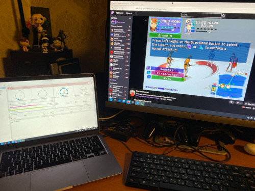
On a Mac with an Apple Silicon processor, you cannot install Linux in the usual way: booting from a flash drive is impossible here, and the bootloader is signed by Apple. The Asahi Linux project undertook to get around this – its participants used reverse engineering to make the M1 and M2 hardware work under regular Linux. Now the flagship distribution of the project is Fedora Asahi Remix, and it works quite reliably on the M2. In this post I will describe the installation step by step.

What is Asahi Linux

The project started in 2020, when Apple switched to its own chips and with them came a closed boot scheme: the device runs only Apple-signed code. Asahi Linux participants wrote their m1n1 bootloader, on top of which they wrote U-Boot and a UEFI environment. Next, the most common ARM64 system is loaded, but with a linux-asahi kernel, to which drivers for non-standard Apple hardware are added: GPU, video, sound, camera units.

In practice, it looks like this: you run the installer from macOS, it partitions the disk, installs the boot chain and the system. macOS remains in place, you get dual boot and choose your system when you turn it on.

Requirements

• Mac on the M2 chip – MacBook Air, MacBook Pro 13″, as well as 14″ and 16″ with M2 Pro and M2 Max. M1 cars are also supported.
• Current macOS. The installer requires the latest version of the system, so update before starting.
• Free space. Minimum about 30 GB, comfortable – 100 GB or more. The space is cut off from the APFS container and will not come back on its own.
• macOS administrator password. You will need it both during partitioning and when booting into recovery mode for the first time.
• Backup. Disk partitioning is an operation that is best started with a fresh backup.

Step 1. Backup and update

Make a copy via Time Machine or any other method. Update macOS to the latest version available and reboot. If FileVault is enabled, the password for it will still be needed at the boot stage in recovery mode – the installer needs to unlock the drive.

Step 2. Launch the installer

Open Terminal on macOS and run one command:

This is the official installer of the project. It will download itself, check your Mac model and offer to choose a distribution. There is also an option directly for Fedora:

The first option is preferable: it shows which systems are currently available, and it also offers a choice of desktop.

Step 3. Disk partition

The installer will ask for the administrator password and show the current layout. Then the dialogue looks like this:

• Press r to resize the macOS partition.
• Enter the size of the new Linux partition. It can be in gigabytes, it can be as a percentage of the disk, or you can write min – then the smallest possible piece will be cut off.
• Confirm the marking with the letter y. This step is the longest: the system physically moves the data in the APFS container; on a large disk this takes several minutes.
• Press f to point the installer to the newly created free partition.

It is important to understand what is happening: Linux is not installed inside APFS, but on a separate partition next to it. This is why macOS remains untouched, and the rollback is reduced to deleting this section.

Step 4. Selecting distribution and desktop

Next, the installer will offer the system and desktop environment. Fedora Asahi Remix comes with KDE Plasma by default – it is the flagship option that receives updates first. An alternative is GNOME, which is closer in feel to macOS. There is also a minimal image if you don’t need a graphical environment.

Step 5. First boot in recovery mode

After partitioning, the installer will prompt you to continue, and the Mac will shut down. Here comes the most unusual part:

• Wait at least 25 seconds – this is Apple’s requirement to enter recovery mode.
• Hold and hold the power button until boot options appear.
• Select the installation volume and enter your macOS password.

At this step, the boot chain is installed in the service partition: m1n1, U-Boot and UEFI environment. Then the machine will reboot again – hold down the power button again and select a new volume, this time to get into the system. There will be several such reboots, each requiring manual selection: by default, the Mac continues to load macOS.

Step 6. Installing the system

Next, the initial setup wizard starts: system name, user, password, time zone, keyboard layout. After this, the installation itself begins, and it is already coming from the Internet – you will need a stable connection, and in time it takes from fifteen minutes to half an hour.

When the installation is complete, reboot and select Linux from the boot menu. When you log in for the first time, the system will prompt you to complete the setup and update.

What works and what doesn’t

Before installation, you should soberly assess what you will lose. On M2 laptops the situation is as follows:

Works:

• Wi-Fi and Bluetooth – without restrictions.
• Integrated screen and graphics – hardware accelerated, including OpenGL and Vulkan.
• Webcam, microphone, and speakers on MacBook Air and MacBook Pro.
• Sleep mode – works normally.
• Hardware video decoding – players do not load the processor.
• USB ports, including USB 2 and USB 3 via Thunderbolt connectors.

Doesn’t work or works partially:

• Touch ID. Fingerprint is not available in Linux – log in with password.
• Thunderbolt (USB4). Status – in development. Unfortunately, devices that specifically require Thunderbolt will not work.
• External monitor via USB-C. DisplayPort Alt Mode is also in operation. M2 laptops don’t have an HDMI port, so you can’t connect an external screen. Models with M2 Pro and M2 Max have HDMI, and it works. A workaround for USB-C is in the fairydust core section below.
• Hardware video encoding is in the plans, decoding is already in place.

Simply put, it’s a great system for working with code, terminal, browser and local models, but not for an external monitor dock.

External monitor via fairydust core

USB-C image output is available in the experimental fairydust kernel branch from the Asahi Linux team. It takes a long time to assemble it manually, so it’s easier to use the wrapper script from the asahi-fairydust-display project:

cd asahi-fairydust-display
chmod +x asahi-fairydust-build.sh
./asahi-fairydust-build.sh

The script clones the fairydust branch, configures and assembles the kernel, places it next to the standard one and edits GRUB. You need 15 GB of free space, a USB-C → HDMI or DisplayPort adapter and 60–90 minutes to assemble. After the reboot, select the kernel labeled -fairydust in GRUB and insert the adapter into the frontmost USB-C port.

Check after download:

glxinfo | grep "OpenGL renderer"
xrandr

The first command should show the version with the suffix -fairydust, the second should show the Apple M2, not llvmpipe, the third should show the connected DP-1 output.

Reservations. The branch is experimental and not officially supported. The output only works through one USB-C port and does not always survive hot plugging – it’s safer to reboot with the adapter already inserted. The script does not automatically configure the display: the corresponding step in it is disabled because it caused a login loop on Wayland. Updating the stock kernel via dnf rearranges the /boot/dtb symlink, which is why the output may silently stop working – then the build must be repeated.

The standard kernel is not touched: to return, just select it in the GRUB menu.

External drive instead of upgrade

Here’s the good side. The MacBook cannot be upgraded: the memory and storage are soldered onto the board, and their capacity is selected once upon purchase. In macOS, the external drive remains external – the system and applications cannot really be transferred to it.

In Linux, this limitation is removed: an external SSD via USB is a regular block device, and any mount point can be transferred to it via /etc/fstab. If you want to transfer your home directory, Steam library, virtual machine images or local models, please do so. It turns out exactly the upgrade that this car does not have.

It looks like this. First, look at the UUID of the desired partition:

sudo blkid

Then add the line to /etc/fstab:

The transfer itself is done by copying: the data is moved to an external drive, after which it is mounted at the desired point. More often than not, not the entire /home is taken away this way, but individual heavy directories – this way there is less risk.

A couple of caveats. The nofail parameter is worth setting in the options: without it, the system will not boot if the disk is not connected. The speed of a USB drive is still lower than the built-in NVMe, so it’s better to leave space on the internal disk for frequent I/O operations. And there is no need to pull out the disk while moving with directories mounted there – first unmount it.

How to switch between systems

When you turn it on, hold down the power button – the boot menu will appear, it will contain macOS and Linux. You can select the default system in macOS: “System Preferences” → “General” → “System Disk”. Linux also has the corresponding settings, so you can switch in both directions without a terminal.

Links

https://asahilinux.org/fedora/
https://asahilinux.org/docs/
https://asahilinux.org/docs/platform/feature-support/m2/
https://fedoraproject.org/asahi-remix
https://github.com/bharambetejas/asahi-fairydust-display
https://github.com/AsahiLinux/linux/tree/fairydust

Sources

https://asahilinux.org/docs/platform/feature-support/m2/
https://discussion.fedoraproject.org/t/fedora-asahi-remix-installation-guide/
https://github.com/AsahiLinux/docs
https://github.com/bharambetejas/asahi-fairydust-display/blob/main/README.md
https://github.com/bharambetejas/asahi-fairydust-display/blob/main/asahi-fairydust-build.sh

Instructions for installing Ubuntu Server in VirtualBox on a Mac with an ARM64 processor and connecting Guest Additions.

Installing VirtualBox

Download the ARM64 build of VirtualBox, mount the image and transfer VirtualBox.app to Applications.

Configuring a virtual machine

We create a new machine, specify the Linux type and the Ubuntu version (64-bit ARM). In the settings we set:

• TPM – disable
• UEFI – disable
• RAM – 4096 MB.
• Graphics controller – VMSVGA (for VBoxLinuxAdditions).
• Processor – 4 cores.

Installing Ubuntu Server

Mount the Ubuntu Server ISO image for ARM64 into the CD-ROM drive. In the download section, put the optical drive first in the list. We start the machine and go through the installation of Ubuntu Server.

Installing xubuntu-desktop

Install the XFCE graphical environment:

sudo apt update
sudo apt install -y xubuntu-desktop

In the login manager selection dialog, select lightdm.

Reboot the guest system:

sudo reboot

Guest Additions

After the first boot, install packages for building kernel modules:

sudo apt update
sudo apt install -y build-essential linux-headers-$(uname -r)

We mount the disk with Guest Additions through the VirtualBox menu: Devices → Mount Guest Additions disk image. The disk will appear inside the guest in the /media/$USER directory.

Open a terminal in Xubuntu, go to the directory of the mounted disk and run the installer:

cd /media/$USER/*
sudo ./VBoxLinuxAdditions-arm64.run

Reboot the guest system:

sudo reboot

What should work after installation

We check that the kernel modules are loaded:

lsmod | grep vbox

The output should include vboxguest and vboxsf.

Add a shared folder in the machine properties and mount it inside the guest:

sudo mkdir -p /media/sf_shared
sudo mount -t vboxsf shared /media/sf_shared

Working features:

• Shared folders – the host directory is visible inside the guest via vboxsf.
• Shared clipboard – copy text between host and guest.
• Mouse integration – the cursor freely extends outside the machine window.
• Automatic resolution change – the guest screen adjusts to the window size.
• Time synchronization – the guest’s time is adjusted to the host’s time.

Sources

https://www.virtualbox.org/manual/topics/guestadditions.html
https://forums.virtualbox.org/viewtopic.php?t=112886

Claude Code is a console agent from Anthropic that can read project files, edit code, run commands and tests, search the repository, and work with git. The main inconvenience when using it is the cost: long sessions with a lot of context quickly eat up the subscription budget.

There is a solution. DeepSeek provides an endpoint compatible with the Anthropic API. It is enough to change the base address and token, and Claude Code will start working on DeepSeek models, without requiring any reinstallation or patches. In this post I will describe how to set this up on macOS, Linux and Windows.

Why is this needed

The reasons may be different:
– Price. DeepSeek models are noticeably cheaper than Claude, and for routine agent tasks – navigating a project, minor edits, running tests – top quality is not always needed.
– Availability. If you do not have a subscription or payment with an Anthropic card is not available for some reason, DeepSeek becomes a working option.
– Experiments. It’s interesting to compare how different models handle the same codebase in the same environment.

What you need

You need Claude Code installed and the DeepSeek API key. If Claude Code is not already installed, the order is as follows:
1. Install Node.js 18 or later. On Windows, you will additionally need Git for Windows.
2. Install Claude Code itself using the command below.
3. Check the installation.

npm install -g @anthropic-ai/claude-code
claude --version

If the version is displayed, then the installation was successful. The API key is created in your DeepSeek personal account on the keys page.

Configuration via environment variables

All integration comes down to environment variables. For macOS and Linux it looks like this:

export ANTHROPIC_BASE_URL=https://api.deepseek.com/anthropic
export ANTHROPIC_AUTH_TOKEN=ваш_ключ_deepseek

export ANTHROPIC_MODEL=deepseek-flash[1m]
export ANTHROPIC_DEFAULT_OPUS_MODEL=deepseek-flash[1m]
export ANTHROPIC_DEFAULT_SONNET_MODEL=deepseek-flash[1m]
export ANTHROPIC_DEFAULT_HAIKU_MODEL=deepseek-flash
export CLAUDE_CODE_SUBAGENT_MODEL=deepseek-flash

export CLAUDE_CODE_EFFORT_LEVEL=max
export CLAUDE_CODE_AUTO_COMPACT_WINDOW=786432

For Windows in PowerShell the syntax is different, but the variable names are the same:

$env:ANTHROPIC_BASE_URL="https://api.deepseek.com/anthropic"
$env:ANTHROPIC_AUTH_TOKEN="ваш_ключ_deepseek"
$env:ANTHROPIC_MODEL="deepseek-flash[1m]"

Let’s figure out what’s what here. The `ANTHROPIC_BASE_URL` variable redirects requests from Anthropic servers to DeepSeek. `ANTHROPIC_AUTH_TOKEN` substitutes your key. The remaining variables determine which model is used in which role. There are models with the `[1m]` suffix – this is an option with a context window of about a million tokens, which allows the agent to hold significantly more project files at a time. Accordingly, `CLAUDE_CODE_AUTO_COMPACT_WINDOW` is set to the size of this window so that automatic history compression does not work too early.

It is convenient not to export variables manually each time, but to register them in the Claude Code configuration. Then the settings will be picked up automatically upon startup.

{
  "env": {
    "ANTHROPIC_BASE_URL": "https://api.deepseek.com/anthropic",
    "ANTHROPIC_AUTH_TOKEN": "ваш_ключ_deepseek",
    "ANTHROPIC_MODEL": "deepseek-flash[1m]",
    "ANTHROPIC_DEFAULT_HAIKU_MODEL": "deepseek-flash",
    "CLAUDE_CODE_SUBAGENT_MODEL": "deepseek-flash"
  }
}

After that, go to the project directory and run the agent:

cd ваш_проект
claude

Claude Code in VS Code

Claude Code is available not only in the terminal, but also as an extension for VS Code. It is installed in the normal way: open the extensions panel using Cmd+Shift+X, find “Claude Code” and click Install. The expansion is produced by Anthropic itself.

The extension contains its own copy of the CLI, and it reads the same ~/.claude/settings.json file as the terminal version. The settings from the previous section also apply here – but with one caveat, which most often causes confusion.

Input verification occurs before launch

Before starting, the extension checks the credentials from its own `claudeCode.environmentVariables` setting, and not from settings.json. The values ​​from settings.json reach the running process – that is, the API address and selected models are picked up correctly – but they do not pass the extension’s own login check. If you see the login screen even though everything is already working in the terminal, this is the reason.

This can be cured with a few lines in the VS Code settings: duplicate the variables in `claudeCode.environmentVariables` and disable the login request.

{
  "claudeCode.environmentVariables": [
    { "name": "ANTHROPIC_BASE_URL", "value": "https://api.deepseek.com/anthropic" },
    { "name": "ANTHROPIC_AUTH_TOKEN", "value": "ваш_ключ_deepseek" },
    { "name": "ANTHROPIC_MODEL", "value": "deepseek-flash[1m]" }
  ],
  "claudeCode.disableLoginPrompt": true
}

macOS nuance

If you launch VS Code from the Dock or Finder, it does not inherit environment variables from ~/.zshrc. This is standard macOS behavior and is specifically discussed in the Claude Code documentation. That is, `export ANTHROPIC_BASE_URL=…` in your shell for the extension simply will not work – this variable will not be in its environment.

There are two conclusions from this. Firstly, the settings in `claudeCode.environmentVariables` are more reliable than shell variables. Secondly, if you still prefer a shell, launch the editor from the terminal, where the variables are already exported:

code .

What won’t work

On a third-party provider, some extension features are not available because they require a claude.ai account:
– there will be no plan usage bar, voice input and Web tab for cloud sessions;
– logout commands are not shown in the menu;
– `/usage` will show the consumption and number of tokens of the current session instead of plan limits;
– Remote Control does not work if the base address is not Anthropic.

This is expected behavior and not a sign that the setup failed.

Separately, I would like to add that JetBrains has its own plugin, but it is designed differently: it does not contain a built-in CLI, but launches one already installed in the integrated terminal. There are no settings for environment variables, so you should launch the IDE from the terminal with already exported variables.

How DeepSeek understands Claude model names

Claude Code internally refers to models by names like claude-opus, claude-sonnet and claude-haiku. DeepSeek intercepts these names and replaces them with its own:
– everything that starts with claude-opus goes to deepseek-v4-pro;
– everything that starts with claude-sonnet or claude-haiku goes to deepseek-flash;
– the unknown model name is also reduced to deepseek-flash.

This means that even without explicitly specifying the models, the integration will work – but it is better to control explicitly which models and at what tariff will serve the request. That is why in the settings above all roles are written manually.

What to pay attention to

Compatibility is incomplete, and you should know this in advance. DeepSeek simply ignores some of the capabilities of the Anthropic API:

– Caching prompts. The `cache_control` field is not supported. Claude Code actively uses the cache so as not to overpay for sending the same context repeatedly. This will not happen here, so long sessions are more expensive than you would expect from the price per token. Periodically start a new dialogue instead of endlessly continuing the old one.
– Thinking Budget. The `thinking` parameter is supported, but the `budget_tokens` inside it are ignored.
– Miscellaneous. The `top_k`, `service_tier`, `container` fields and the connection of MCP servers from the API are also ignored.
– MCP. The built-in MCP server mechanism on the DeepSeek side does not work, although the agent’s usual tools – reading files, editing, running commands, searching – function normally.

Separately, it is worth mentioning proxies. There are projects in the community like `ds-cc-proxy`, which are placed between Claude Code and DeepSeek and take on the task of smoothing out minor incompatibilities, as well as separating the main session and subagents into different models. If the standard setup behaves unstable, such an intermediate layer can help.

Claude Code Router

The method described above puts one model on all tasks. But the agent does very different things: he understands the structure of the project, corrects little things, and sometimes solves a truly complex problem. It is logical that different models should be used for different types of work. This is exactly what the claude-code-router (CCR) can do – a local gateway that stands between Claude Code and model providers.

What does it give

– Routing by rules. You can set which model serves the main session, which one serves background tasks, which one serves the scheduling mode. It makes sense to use an expensive model only for complex reasoning, and to give away the routine to a cheap one.
– Backup options. If the provider returns an error, the request goes to the next model in the chain, rather than dropping the session.
– Observability. The interface shows the request log, delays, token consumption and cost – something that you can only guess about with a direct connection.
– One address for several agents. Providers, keys and rules live in one place, and clients connect to one local address.

First about versions – this is important

It’s worth warning here because it will save you time. CCR has been heavily redesigned over its history, and almost all the articles you find in a search describe the outdated version.

In older versions, the configuration was in the file ~/.claude-code-router/config.json with the Providers and Router blocks, and everything was launched with the `ccr code` command. Now it doesn’t work that way anymore. The current version (3.x) stores settings in the SQLite database and is managed via a web interface. The old config.json is read exactly once as a source for migration if there is no database yet – after that, edits to it do not affect anything.

That is, if you found instructions on the Internet with editing config.json and the `ccr code` command and nothing worked for you, you are editing a file that no one reads anymore. It’s not your fault.

Installation

You will need Node.js 22 or later.

npm install -g @musistudio/claude-code-router
ccr ui

The `ccr ui` command brings up the service in the background and opens the management interface in the browser. It is useful to know the other commands: `ccr start` starts a service, `ccr stop` stops it, `ccr serve` works in the foreground and is convenient when you need to see logs.

By default, the management interface lives on port 3458, and the gateway itself for models lives on port 3456.

Settings

Everything is done in the web interface, without manually editing files:
1. In the Providers section, add the DeepSeek provider and specify its key. Please note: the full address up to the chat/completions point is needed here, not just the domain.
2. In the Models section, describe what this model is – the description helps routing.
3. In the Agent Config section, set the default model.
4. In the Routing section, configure the rules: which model responds to which requests.
5. On the API Keys page, create a CCR client key – this is what Claude Code will use, not the DeepSeek key.

After this, all that remains is to send Claude Code to the gateway: specify the gateway address shown in the interface as the base address, and the CCR client key as the token.

A nice thing: routing rules can be written not only with fields, but also with a JavaScript script, if the logic is more complex than comparing one field.

Is it worth using it

Connecting DeepSeek to Claude Code is primarily a way to reduce costs without giving up a convenient agent environment. You get the same interface, the same tools, and the same workflow, but on a different model. The setup takes a few minutes and is completely reversible: just remove the environment variables to return to Anthropic models.

The limitations are also clear: there is no prompt cache, incomplete compatibility with respect to API fields, and the quality of the model may differ for complex architectural tasks. For routine work in the repository – navigation, refactoring, running tests – this is more than enough.

Example: Oni-Extended

A living example of such a combination is my project Oni-Extended, a fork of the port of the game Oni (Bungie, 2001) for Apple Silicon. The game sources are written in C and have been around for more than twenty years; there have never been any tests in them, and the file sizes are measured in tens of thousands of lines. However, new features have been added to the project via Claude Code from DeepSeek: fast saving and loading via F5/F9, a key hold block, and a -nodamage launch flag that disables damage.

This is a good illustration of what was said above. All tasks relate to routine work in a large repository – the agent examines other people’s code, finds connections between modules and tests hypotheses, rather than designing an architecture from scratch. The cost of such sessions on DeepSeek turns out to be noticeably lower than on Anthropic models, despite the fact that the result is verified by the project’s own infrastructure: assembly, level run stand and offline tests.

Links

https://platform.deepseek.com/api_keys
https://api-docs.deepseek.com
https://docs.anthropic.com/en/docs/claude-code
https://github.com/anthropics/claude-code
https://github.com/musistudio/claude-code-router
https://ccrdesk.top/en/guides/cli/
https://github.com/zefir1990/Oni-Extended

Sources

https://api-docs.deepseek.com/guides/anthropic_api
https://api-docs.deepseek.com/quick_start/agent_integrations/claude_code
https://ccrdesk.top/en/routing/
https://code.claude.com/docs/en/vs-code

Donki Hills has been on Steam for over a year now!

Exactly a year ago the project appeared on the Steam page, and since then the game has come a long way. During this time, there were many experiments, changes and searches for the very direction in which Donki Hills should develop.

Work on the gameplay continues, and now the project is gradually acquiring its true face. Donki Hills is starting to turn into what it was intended to be – Comedy First Person Roguelike Parody Survival Horror.

A strange adventure where horror meets humor, exploration and unexpected situations. You have to go to the city, look for objects, solve riddles and gradually uncover the secret that will lead you to Maria.

Below are fresh screenshots from the next playtest of the prototype. This is not the final look of the game yet, but you can already feel the atmosphere of the city and the direction in which the project is moving.

Very interested to hear your reaction! 👀
How do you like the new direction? What are your impressions of the atmosphere and ideas of the game?

Thanks to everyone who added Donki Hills to their wishlist, follows the development and supports the project ❤️

There are still many experiments, new mechanics and strange adventures ahead.

https://store.steampowered.com/app/3476390/Donki_Hills/

Manufacturers of modern gaming laptops often configure systems so that the processor warms up to 90 degrees and even reaches 100 degrees Celsius under load. This problem is especially acute in the summer when running demanding games or heavy work tasks.

Due to extreme heating, throttling is activated (resetting the processor frequencies to prevent physical damage), which leads to a sharp loss of performance, freezes and a drop in FPS. There are many ways to combat overheating (from using cooling pads to undervolting), but in this article I will describe the simplest and fastest method that is relevant for Windows 11 and earlier versions of the operating system.

The method is to limit the maximum processor state through power supply settings:

1. Open Power Options via Windows Search or Control Panel.
2. In the active power plan, go to the section for changing additional parameters.
3. Find the Processor power management branch.
4. Expand the Maximum processor state option.
5. For Plugged In, change the value from 100% to 80% or less.

After applying these settings, the processor will no longer automatically overclock to extreme frequencies that generate excess heat. Although the maximum peak performance will decrease by approximately 20%, the processor will no longer overheat. Stable operation at a reduced frequency without throttling is MUCH better and more comfortable for the system than constant sharp jumps in performance due to overheating at temperatures under 100 degrees.

Each laptop is unique, so I recommend that users experiment and find the optimal balance (percentage) that will provide the desired performance without overheating.

In this post I will describe how I ported the Surreal Engine game engine to WebAssembly.
https://demensdeum.com/demos/SurrealEngine/”
Surreal Engine – a game engine that implements most of the functionality of the Unreal Engine 1, famous games on this engine – Unreal Tournament 99, Unreal, Deus Ex, Undying. It refers to classic engines that worked primarily in a single-threaded execution environment.
I originally had the idea of ​​taking on a project that I couldn’t complete in any reasonable time frame, thus showing my Twitch followers that there are projects that even I can’t do. During my first stream, I suddenly realized that the task of porting Surreal Engine C++ to WebAssembly using Emscripten was feasible.

A month later, I can demonstrate my fork and engine assembly on WebAssembly:
https://demensdeum.com/demos/SurrealEngine/
Control, as in the original, is carried out using the keyboard arrows. Next, I plan to adapt it for mobile control (tachi), adding correct lighting and other graphic features of the Unreal Tournament 99 render.

Where to start?

The first thing I want to say is that any project can be ported from C++ to WebAssembly using Emscripten, the only question is how complete the functionality will be. Choose a project whose library ports are already available for Emscripten; in the case of Surreal Engine, you are very lucky, because the engine uses the SDL 2, OpenAL – libraries. they are both ported to Emscripten. However, Vulkan is used as a graphics API, which is currently not available for HTML5, work is underway to implement WebGPU, but it is also in the draft stage, and it is also unknown how simple the further port from Vulkan to WebGPU will be, after it is fully standardized. Therefore, I had to write my own basic OpenGL-ES / WebGL renderer for Surreal Engine.

Building the project

Build system in Surreal Engine – CMake, which also simplifies porting, because Emscripten provides its native builders – emcmake, emmake.
The Surreal Engine port was based on the code of my latest game in WebGL/OpenGL ES and C++ called Death-Mask, because of this the development was much simpler, I had all the necessary build flags with me and code examples.
One of the most important points in CMakeLists.txt is the build flags for Emscripten, below is an example from the project file:

set(CMAKE_CXX_FLAGS "-s MIN_WEBGL_VERSION=2 
-s MAX_WEBGL_VERSION=2 
-s EXCEPTION_DEBUG 
-fexceptions 
--preload-file UnrealTournament/ 
--preload-file SurrealEngine.pk3 
--bind 
--use-preload-plugins 
-Wall 
-Wextra 
-Werror=return-type 
-s USE_SDL=2 
-s ASSERTIONS=1 
-w 
-g4 
-s DISABLE_EXCEPTION_CATCHING=0 
-O3 
--no-heap-copy 
-s ALLOW_MEMORY_GROWTH=1 
-s EXIT_RUNTIME=1")

The build script itself:

clear
emmake make -j 16
cp SurrealEngine.data /srv/http/SurrealEngine/SurrealEngine.data
cp SurrealEngine.js /srv/http/SurrealEngine/SurrealEngine.js
cp SurrealEngine.wasm /srv/http/SurrealEngine/SurrealEngine.wasm
cp ../buildScripts/Emscripten/index.html /srv/http/SurrealEngine/index.html

Next, let’s prepare index.html, which includes the project file system preloader. To upload to the web, I used Unreal Tournament Demo version 338. As you can see from the CMake file, the unpacked game folder was added to the build directory and linked as a preload-file for Emscripten.

Main code changes

Then we had to change the game loop of the game, you can’t run an endless loop, this leads to the browser freezing, instead you need to use emscripten_set_main_loop, I wrote about this feature in my 2017 note “Porting SDL C++ games to HTML5 (Emscripten)”
We change the code for exiting the while loop to if, then we display the main class of the game engine, which contains the game loop, in the global scope, and write a global function that will call the game loop step from the global object:

#if __EMSCRIPTEN__
#include <emscripten.h>
Engine *EMSCRIPTEN_GLOBAL_GAME_ENGINE = nullptr;
void emscripten_game_loop_step() {
	EMSCRIPTEN_GLOBAL_GAME_ENGINE->Run();
}
#endif

After this, you need to make sure that there are no background threads in the application; if there are, then get ready to rewrite them for single-threaded execution, or use the phtread library in Emscripten.
The background thread in Surreal Engine is used to play music, data comes from the main engine thread about the current track, the need to play music, or its absence, then the background thread receives a new state via a mutex and starts playing new music, or pauses. The background thread is also used to buffer music during playback.
My attempts to build Surreal Engine for Emscripten with pthread were unsuccessful, because the SDL2 and OpenAL ports were built without pthread support, and I didn’t want to rebuild them for the sake of music. Therefore, I transferred the functionality of the background music stream to single-threaded execution using a loop. By removing pthread calls from the C++ code, I moved the buffering and music playback to the main thread, so that there would be no delays, I increased the buffer by a few seconds.
Next, I will describe specific implementations of graphics and sound.

Vulkan is not supported!

Yes, Vulkan is not supported in HTML5, although all the marketing brochures present cross-platform and broad platform support as the main advantage of Vulkan. For this reason, I had to write my own basic graphics renderer for a simplified OpenGL type – ES, it is used on mobile devices, sometimes it does not contain the fashionable features of modern OpenGL, but it ports very well to WebGL, which is exactly what Emscripten implements. Writing basic tile rendering, bsp rendering, for the simplest GUI display, and rendering models + maps was completed in two weeks. This was perhaps the most difficult part of the project. There is still a lot of work ahead to implement the full functionality of Surreal Engine rendering, so any help from readers is welcome in the form of code and pull requests.

OpenAL supported!

The big luck is that Surreal Engine uses OpenAL for audio output. Having written a simple hello world in OpenAL and assembled it in WebAssembly using Emscripten, it became clear to me how simple everything was, and I set off to port the sound.
After several hours of debugging, it became obvious that the OpenAL implementation of Emscripten has several bugs, for example, when initializing reading the number of mono channels, the method returned an infinite number, and after trying to initialize a vector of infinite size, C++ crashes with the exception vector::length_error.
We managed to get around this by hardcoding the number of mono channels to 2048:

		alcGetIntegerv(alDevice, ALC_MONO_SOURCES, 1, &monoSources);
		alcGetIntegerv(alDevice, ALC_STEREO_SOURCES, 1, &stereoSources);

#if __EMSCRIPTEN__
		monoSources = 2048; // for some reason Emscripten's OpenAL gives infinite monoSources count, bug?
#endif

Is there a network?

Surreal Engine does not currently support online play, play with bots is supported, but we need someone to write AI for these bots. Theoretically, you can implement a network game on WebAssembly/Emscripten using Websockets.

Conclusion

In conclusion, I would like to say that the porting of Surreal Engine turned out to be quite smooth due to the use of libraries for which there are Emscripten ports, as well as my past experience in implementing a game in C++ for WebAssembly on Emscripten. Below are links to sources of knowledge and repositories on the topic.
M-M-M-MONSTER KILL!
Also, if you want to help the project, preferably with WebGL/OpenGL ES rendering code, then write to me in Telegram:
https://t.me/demenscave

Links

https://demensdeum.com/demos/SurrealEngine/

https://github.com/demensdeum/SurrealEngine-Emscripten

https://github.com/dpjudas/SurrealEngine

When two devices are behind NAT or strict firewalls and cannot “see” each other directly, a VPN seems to be the standard solution. But a full-fledged L3 tunnel (like WireGuard or OpenVPN) is often redundant: it requires root rights, setting up virtual interfaces, and can conflict with existing routes.

In such cases, it is convenient to use Chisel – a TCP/UDP tunnel that runs on top of HTTP and uses WebSockets for data transfer. In this note I will show how to “forward” a port from one client to another through an intermediate server.

How does it work?

Imagine the situation: you have Client A (for example, your home server), Client B (your work laptop) and a VPS with a public IP address. Clients A and B can access the VPS, but not each other.

The forwarding scheme will look like this:
1. Client A connects to the VPS and opens a “reverse” port on the server. Now everything that comes to port X of the server goes to port Y of Client A.
2. Client B connects to the VPS and forwards port Z from its local machine to port X of the server.
3. As a result, Client B accesses localhost:Z and ends up on Client A:Y.

This approach is one of the solutions in cases where communication with a VPS does not implement an L3 layer or there is no ability to configure routing between clients. We work exclusively at the application and port level.

Step 1: Start the server

On your VPS, just run Chisel in server mode. The --reverse flag is required to allow clients to open ports on the server side.

chisel server --port 8080 --reverse

Step 2: Connecting Client A (Source)

Let’s say Client A wants to open access to his local web server on port 3000. He connects to the VPS and says: “reserve port 2000 on the server and forward it to me to 3000.”

chisel client vps-ip:8080 R:2000:127.0.0.1:3000

Now port 2000 on the VPS (on the loopback interface) leads to Client A.

Step 3: Connecting Client B (Consumer)

Now Client B wants to access this resource. It connects to the same VPS and forwards its local port 8080 to port 2000 of the server.

chisel client vps-ip:8080 8080:127.0.0.1:2000

Ready! Now, when you open http://localhost:8080 on Client B, you will see the service running on Client A.

Safety and nuances

Chisel supports authentication via the --auth flag, which is highly recommended when working through public servers. You can also use TLS certificates to encrypt traffic.

The main advantage of this approach is that there is no need for TUN/TAP devices and complex routing tables. This is a stripped-down tunnel that does exactly one thing: binds ports via a WebSocket connection. This even works through corporate proxies if you configure Chisel to work through port 443.

Output

Chisel is a utility for specific network tasks. When you need to forward ports between isolated nodes without setting up a full-fledged VPN, a combination of forward and reverse tunnels through a relay server turns out to be a completely viable solution.

Links

https://github.com/jpillora/chisel

You spend hours working on the code, going through hypotheses, adjusting the conditions, but the bug is still reproduced. Sound familiar? This state of frustration is often called “ghost hunting.” The program seems to live its own life, ignoring your corrections.

One of the most common – and most annoying – reasons for this situation is looking for an error in completely the wrong place in the application.

The trap of “false symptoms”

When we see an error, our attention is drawn to the place where it “shot”. But in complex systems, where a bug occurs (crash or incorrect value) is only the end of a long chain of events. When you try to fix the ending, you are fighting the symptoms, not the disease.

This is where the flowchart concept comes in.

How it works in reality

Of course, it is not necessary to directly draw (draw) a flowchart on paper every time, but it is important to have it in your head or at hand as an architectural guide. A flowchart allows you to visualize the operation of an application as a tree of outcomes.

Without understanding this structure, the developer is often groping in the dark. Imagine the situation: you edit the logic in one condition branch, while the application (due to a certain set of parameters) goes to a completely different branch that you didn’t even think about.

Result: You spend hours on a “perfect” code fix in one part of the algorithm, which, of course, does nothing to fix the problem in another part of the algorithm where it actually fails.

Algorithm for defeating a bug

To stop beating on a closed door, you need to change your approach to diagnosis:

• Find the state in the outcome tree:Before writing code, you need to determine exactly the path that the application has taken. At what point did logic take a wrong turn? What specific state (State) led to the problem?
• Reproduction is 80% of success: This is usually done by testers and automated tests. If the bug is “floating”, development is involved in the process to jointly search for conditions.
• Use as much information as possible: Logs, OS version, device parameters, connection type (Wi-Fi/5G) and even a specific telecom operator are important for localization.

“Photograph” of the moment of error

Ideally, to fix it, you need to get the full state of the application at the time the bug was reproduced. Interaction logs are also critically important: they show not only the final point, but also the entire user path (what actions preceded the failure). This helps to understand how to recreate a similar state again.

Future tip: If you encounter a complex case, add extended debug logging information to this section of code in case the situation happens again.

The problem of “elusive” states in the era of AI

In modern systems using LLM (Large Language Models), classical determinism (“one input, one output”) is often violated. You can pass exactly the same input data, but get a different result.

This happens due to the non-determinism of modern production systems:

• GPU Parallelism: GPU floating point operations are not always associative. Due to parallel execution of threads, the order in which numbers are added may change slightly, which may affect the result.
• GPU temperature and throttling: Execution speed and load distribution may depend on the physical state of the hardware. In huge models, these microscopic differences accumulate and can lead to the selection of a different token at the output.
• Dynamic batching: In the cloud, your request is combined with others. Different batch sizes change the mathematics of calculations in the kernels.

Under such conditions, it becomes almost impossible to reproduce “that same state”. Only a statistical approach to testing can save you here.

When logic fails: Memory problems

If you are working with “unsafe” languages ​​(C or C++), the bug may occur due to Memory Corruption.

These are the most severe cases: an error in one module can “overwrite” data in another. This leads to completely inexplicable and isolated failures that cannot be traced using normal application logic.

How to protect yourself at the architectural level?

To avoid such “mystical” bugs, you should use modern approaches:

• Multithreaded programming patterns:Clear synchronization eliminates race conditions.
• Thread-safe languages: Tools that guarantee memory safety at compile time:
  • Rust: Ownership system eliminates memory errors.
  • Swift 6 Concurrency:Strong data isolation checks.
  • Erlang: Complete process isolation through the actor model.

Summary

Fixing a bug is not about writing new code, but about understanding how the old one works. Remember: you could be wasting time editing a branch that management doesn’t even touch. Record the state of the system, take into account the factor of AI non-determinism and choose safe tools.

(and how to create solutions that continue to work after updates)

“Apps may only use public APIs and must run on the currently shipping OS.” Apple App Review Guidelines

If you’ve ever started working with a new framework and found yourself thinking: “Now I’ll understand everything myself, reading the documentation is too long,” you’re definitely not alone. Many of us have a natural investigative instinct: try first, and only then look at the instructions. And that’s completely normal.

However, at this stage it can be easy to get carried away and end up in a situation where the code works great, but perhaps relies on non-obvious features of the system.

Why is it sometimes not enough to simply “figure it out on your own”?

Frameworks, especially closed ones, are complex and multi-layered systems. They often hide internal logic and optimizations that:

* are not described in public documentation;
* do not guarantee that behavior will be maintained in the future;
* may change with the release of new versions;
* may contain features known to the developers that have not yet been fixed.

When we act intuitively, there is a risk of building architecture on random observations rather than on documented rules. This can make the code more sensitive to updates.

Documentation is not a limitation, but a reliable support

Framework developers create manuals to help us. Acting within the documentation, we get:

* stability;
* support;
* predictable system behavior.

By going beyond these limits, we take on additional risks, and maintaining such code becomes more difficult.

Experiments? Certainly. But with an understanding of boundaries.
Curiosity is a great trait to have in a developer. Exploring and trying new things is absolutely essential. But here is a small wish:

The most comfortable way to experiment is to rely on best practices.

The documentation is a map that shows which paths are the most secure and supported by the creators.

An outside perspective: expert advice

We often learn from experienced colleagues:

* they conduct useful courses,
* speak at conferences,
* write wonderful books and blogs,
* share their unique vision.

Many of them share truly valuable experiences. But it is worth remembering: if the author’s approaches contradict the official documentation, they may turn out to be fragile.

Such “empirical patterns” sometimes:

* work only on a specific version of the framework;
* sensitive to updates;
* may behave unpredictably in unusual situations.

Learning from the community is great and rewarding. But any advice, even the most authoritative, should always be carefully checked with official manuals.

A little about SOLID

Three ideas from the SOLID principles perfectly complement this approach:

* Open/Closed Principle: Try to extend behavior through public APIs and, if possible, not depend on hidden implementation.
* Liskov Substitution Principle: Rely on the contract, not the specific implementation. Otherwise, changes under the hood can lead to unexpected difficulties.
* Dependency Inversion: build dependencies on abstractions, not details.

In practice, this means that being tied to internal, undocumented details of the framework makes the system brittle.
Based on public interfaces and contracts, we get:

* better isolation of code from changes in the framework;
* ease of testing;
* predictability and reliability of the architecture.

What if there is a bug?

It also happens that everything is done according to the rules, but the result does not meet expectations. Frameworks evolve and are not always perfect. In such cases:

* Build a minimal example that reproduces the problem.
* Ensure that only documented APIs are used.
* Send a bug report – the development team will certainly appreciate your work and try to help.

If the example relies on workarounds, it will be much more difficult for developers to provide support.

How to get the most out of the framework

*Refer to documentation.
* Follow the guides and recommendations of the authors.
* Experiment within the described functionality.
* Check advice from the Internet with official sources.
* Localize bugs while respecting framework contracts.

Conclusion

Frameworks are powerful tools with their own rules of the game. By forgetting about them, we risk making our code overly vulnerable. But we all want the created products to live for a long time and not require urgent corrections after each minor update.

Manuals and documentation are excellent support that helps create truly reliable solutions.

Sources

https://developer.apple.com/app-store/review/guidelines/
https://en.wikipedia.org/wiki/SOLID
https://en.wikipedia.org/wiki/API
https://en.wikipedia.org/wiki/RTFM

In this note, I will describe the procedure for building a C++ SDL application for iOS on Linux, signing an ipa archive without a paid Apple Developer subscription, and installing it on a clean device (iPad) using macOS without Jailbreak.

First, let’s install the build toolchain for Linux:
https://github.com/tpoechtrager/cctools-port

The toolchain needs to be downloaded from the repository, then follow the instructions on the Godot Engine website to complete the installation:
https://docs.godotengine.org/ru/latest/development/compiling/cross-compiling_for_ios_on_linux.html

At the moment, you need to download Xcode dmg and copy the sdk from there to build cctools-port. This stage is easier to complete on macOS; just copy the necessary sdk files from the installed Xcode. After successful assembly, the terminal will contain the path to the cross-compiler toolchain.
Next, you can start building the SDL application for iOS. Let’s open cmake and add the necessary changes to build the C++ code:

SET(CMAKE_SYSTEM_NAME Darwin)
SET(CMAKE_C_COMPILER arm-apple-darwin11-clang)
SET(CMAKE_CXX_COMPILER arm-apple-darwin11-clang++)
SET(CMAKE_LINKER arm-apple-darwin11-ld)

Now you can compile using cmake and make, but do not forget to add $PATH to the cross-compiler toolchain:

PATH=$PATH:~/Sources/cctools-port/usage_examples/ios_toolchain/target/bin

For correct linking with frameworks and SDL, we write them in cmake, dependencies of the game Space Jaguar for example:

target_link_libraries(
${FSEGT_PROJECT_NAME}
${FLAME_STEEL_PROJECT_ROOT_DIRECTORY}/scripts/buildScripts/ios/resources/libs/libclang_rt.ios.a
${FLAME_STEEL_PROJECT_ROOT_DIRECTORY}/scripts/buildScripts/ios/resources/libs/libSDL2.a
${FLAME_STEEL_PROJECT_ROOT_DIRECTORY}/scripts/buildScripts/ios/resources/libs/libSDL2_mixer.a
${FLAME_STEEL_PROJECT_ROOT_DIRECTORY}/scripts/buildScripts/ios/resources/libs/libSDL2_image.a
"${FLAME_STEEL_PROJECT_ROOT_DIRECTORY}/scripts/buildScripts/ios/resources/libs/CoreServices.framework"
"${FLAME_STEEL_PROJECT_ROOT_DIRECTORY}/scripts/buildScripts/ios/resources/libs/ImageIO.framework"
"${FLAME_STEEL_PROJECT_ROOT_DIRECTORY}/scripts/buildScripts/ios/resources/libs/Metal.framework"
"${FLAME_STEEL_PROJECT_ROOT_DIRECTORY}/scripts/buildScripts/ios/resources/libs/AVFoundation.framework"
"${FLAME_STEEL_PROJECT_ROOT_DIRECTORY}/scripts/buildScripts/ios/resources/libs/GameController.framework"
"${FLAME_STEEL_PROJECT_ROOT_DIRECTORY}/scripts/buildScripts/ios/resources/libs/CoreMotion.framework"
"${FLAME_STEEL_PROJECT_ROOT_DIRECTORY}/scripts/buildScripts/ios/resources/libs/CoreGraphics.framework"
"${FLAME_STEEL_PROJECT_ROOT_DIRECTORY}/scripts/buildScripts/ios/resources/libs/AudioToolbox.framework"
"${FLAME_STEEL_PROJECT_ROOT_DIRECTORY}/scripts/buildScripts/ios/resources/libs/CoreAudio.framework"
"${FLAME_STEEL_PROJECT_ROOT_DIRECTORY}/scripts/buildScripts/ios/resources/libs/QuartzCore.framework"
"${FLAME_STEEL_PROJECT_ROOT_DIRECTORY}/scripts/buildScripts/ios/resources/libs/OpenGLES.framework"
"${FLAME_STEEL_PROJECT_ROOT_DIRECTORY}/scripts/buildScripts/ios/resources/libs/UIKit.framework"
"${FLAME_STEEL_PROJECT_ROOT_DIRECTORY}/scripts/buildScripts/ios/resources/libs/Foundation.framework"
)

In my case, the SDL, SDL_Image, SDL_mixer libraries are compiled in Xcode on macOS in advance for static linking; Frameworks copied from Xcode. Also added is the libclang_rt.ios.a library, which includes iOS-specific runtime calls, for example isOSVersionAtLeast. Included a macro for working with OpenGL ES, disabling unsupported functions in the mobile version, similar to Android.
After solving all the build problems, you should get the assembled binary for arm. Next, let’s consider running the assembled binary on a device without Jailbreak.
On macOS, install Xcode, register on the Apple portal, without paying for the developer program. Add an account in Xcode -> Preferences -> Accounts, create a blank application and build on a real device. During assembly, the device will be added to your free developer account. After assembly and launch, you need to build the archive; to do this, select Generic iOS Device and Product -> Archive. Once the archive is built, extract the embedded.mobileprovision and PkgInfo files from it. From the build log to the device, find the codesign line with the correct signature key, the path to the entitlements file with the extension app.xcent, copy it.
Copy the .app folder from the archive, replace the binary in the archive with one compiled by a cross-compiler in Linux (for example, SpaceJaguar.app/SpaceJaguar), then add the necessary resources to the .app, check the integrity of the PkgInfo and embedded.mobileprovision files in the .app from the archive, copy again if necessary. We re-sign the .app using the codesign command – codesign requires an input key for sign, the path to the entitlements file (can be renamed with a .plist extension)
After re-signing, create a Payload folder, move the folder with the .app extension there, create a zip archive with Payload in the root, rename the archive with the .ipa extension. After that, in Xcode, open the list of devices and Drag’n’Drop the new ipa to the device’s list of applications; Installation via Apple Configurator 2 does not work for this method. If the re-signing is done correctly, then the application with the new binary will be installed on an iOS device (for example, iPad) with a 7-day certificate, this is enough for the testing period.

Sources

https://github.com/tpoechtrager/cctools-port

https://docs.godotengine.org/ru/latest/development/compiling/cross-compiling_for_ios_on_linux.html

https://jonnyzzz.com/blog/2018/06/13/link-error-3/

https://stackoverflow.com/questions/6896029/re-sign-ipa-iphone

https://developer.apple.com/library/archive/documentation/Security/Conceptual/CodeSigningGuide/Procedures/Procedures.html

In this post I will describe the process of building libraries and applications for Windows using the MinGW32 toolchain on Ubuntu.
Install wine, mingw:

sudo apt-get install wine mingw-w64

After this, you can already build C/C++ applications for Windows:

# C
i686-w64-mingw32-gcc helloWorld.c -o helloWorld32.exe      # 32-bit
x86_64-w64-mingw32-gcc helloWorld.c -o helloWorld64.exe    # 64-bit
 
# C++
i686-w64-mingw32-g++ helloWorld.cc -o helloWorld32.exe     # 32-bit
x86_64-w64-mingw32-g++ helloWorld.cc -o helloWorld64.exe   # 64-bit

The collected exe can be checked using wine.
Next, let’s look at the changes to the CMake build, the CMakeLists.txt file, adding MinGW specific things to the build file:

if (MINGW32)
set(CMAKE_SYSTEM_NAME Windows)
SET(CMAKE_C_COMPILER i686-w64-mingw32-gcc)
SET(CMAKE_CXX_COMPILER i686-w64-mingw32-g++)
SET(CMAKE_RC_COMPILER i686-w64-mingw32-windres)
set(CMAKE_RANLIB i686-w64-mingw32-ranlib)
endif()

// для сборки shared dll
elseif (MINGW32)
add_library(FlameSteelEngineGameToolkit.dll SHARED ${SOURCE_FILES})
else()

// обязательно линкуем со всеми зависимостями
if (MINGW32)
target_link_libraries(
                        FlameSteelEngineGameToolkit.dll 
                        -static-libgcc
                        -static-libstdc++
                        SDL2 
                        SDL2_mixer 
                        /home/demensdeum/Sources/cube-art-project-bootstrap/FlameSteelFramework/FlameSteelCore/FlameSteelCore.dll
                        /home/demensdeum/Sources/cube-art-project-bootstrap/FlameSteelFramework/FlameSteelBattleHorn/FlameSteelBattleHorn.dll
                        /home/demensdeum/Sources/cube-art-project-bootstrap/FlameSteelFramework/FlameSteelCommonTraits/FlameSteelCommonTraits.dll)

set_target_properties(FlameSteelEngineGameToolkit.dll PROPERTIES
        PREFIX ""
        SUFFIX ""
        LINK_FLAGS "-Wl,--add-stdcall-alias"
        POSITION_INDEPENDENT_CODE 0 # this is to avoid MinGW warning; 
        # MinGW generates position-independent-code for DLL by default
)
else()

We collect:

cmake -DMINGW32=1 .
make

The output will be a dll or exe, depending on what you are collecting. For a working example, you can look at the repository of the new Cube-Art-Project and its libraries:
https://gitlab.com/demensdeum/cube-art-project

https://gitlab.com/demensdeum/FlameSteelEngineGameToolkitFSGL

https://gitlab.com/demensdeum/cube-art-project-bootstrap

Sources
https://arrayfire.com/cross-compile-to-windows-from-linux/

In this post, I will describe building cross-platform C++ applications for macOS on an Ubuntu build machine using CMake and osxcross.
First, install the osxcross toolchain:
https://github.com/tpoechtrager/osxcross
Installation occurs in 3 stages, downloading dependencies:

cd tools
./get_dependencies.sh

Download XCode.xip from the official Apple website, then download the SDK from XCode:

./gen_sdk_package_pbzx.sh /media/demensdeum/2CE62A79E62A4404/LinuxSupportStorage/xcode111.xip

I hope you read the XCode license agreement in the last step? Next, build the toolchain with the required prefix:

INSTALLPREFIX=/home/demensdeum/Apps/osxcross ./build.sh 

Now you can use osxcross from the prefix directory of the previous step. Let’s add a new build macro for CMake and write everything necessary:

if (OSXCROSS)
SET(CMAKE_SYSTEM_NAME Darwin)
SET(CMAKE_C_COMPILER o64-clang)
SET(CMAKE_CXX_COMPILER o64-clang++)
SET(CMAKE_C_COMPILER_AR x86_64-apple-darwin19-ar)
SET(CMAKE_CXX_COMPILER_AR x86_64-apple-darwin19-ar)
SET(CMAKE_LINKER x86_64-apple-darwin19-ld)
SET(ENV{OSXCROSS_MP_INC} 1)
endif()

Dynamic linking was not successful for me, so we export the libraries statically:

if (OSXCROSS)
add_library(FlameSteelCore STATIC ${SOURCE_FILES})
else()

Next, you may be faced with the fact that you do not have the necessary libraries for osxcross, I encountered this when using SDL2. osxcross supports ready-made library packages – macports. For example, installing SDL2-mixer:

osxcross-macports -v install libsdl2_mixer

After this, you can start building libraries/applications as usual in the cmake-make link, do not forget to specify static linking of libraries if necessary.

Manual assembly of libraries

Currently, I have encountered the problem of incorrect archiving of libraries during static linking; when building the final application I receive the error:

file was built for archive which is not the architecture being linked (x86_64)

Very similar to this ticket, we managed to implement a workaround resulting in the build completing correctly. Let’s unzip the static library and build it anew using the osxcross archiver:

ar x ../libFlameSteelCore.a
rm ../libFlameSteelCore.a
x86_64-apple-darwin19-ar rcs ../libFlameSteelCore.a *.o

Also, one of the problems I personally consider is the lack of ability to run macOS applications directly on Ubuntu (at least with part of the functionality). Of course, there is a project darling, but the support still leaves much to be desired.

Sources

https://github.com/tpoechtrager/osxcross

Nowadays, you don’t have to rely on cloud services: you can generate high-quality images entirely on your own hardware. In this post, I will describe how to run the modern FLUX model locally on your computer using ComfyUI.

ComfyUI uses node-based architecture. This allows you to:
– Totally control every stage of generation.
– Easily share ready-made “workflows”

FLUX is a large model, so the hardware requirements are higher than SD 1.5 or SDXL:
– Video card (GPU): Nvidia RTX with 12 GB VRAM or higher (for comfortable work). If you have 8 GB or less, you will have to use the quantized versions (GGUF or NF4).
– Random access memory (RAM): minimum 16 GB (preferably 32 GB and above).
– Disk Space: Approximately 20–50 GB for models and components.

The easiest way to start FLUX is to use a ready-made template. Just search for flux text to image in the workflows window and install.

Write a prompt in English in the `Text to Image (Flux.1 Dev)` node, select the resolution (FLUX works well with 1024×1024 and even higher) and press RUN.

The first generation may take time as the models will be loaded into the video card memory.

https://github.com/comfyanonymous/ComfyUI

If you had a desire to use neural networks to help write code (so-called Vibe coding), and you have a fairly powerful computer, for example with an Nvidia RTX video card, then you can deploy the entire environment absolutely free on your machine. This solves problems with paid subscriptions and allows you to safely work with projects under NDA, since your code is not sent anywhere. In this post I will describe how to assemble a local bundle of LM Studio, VS Code and the Continue extension.

Tools for local Vibe coding

For comfortable work we need three main components:
– LM Studio: a convenient application for downloading and running local LLMs. It takes on all the complexity of working with GGUF models and puts up a local server compatible with the OpenAI API.
– VS Code: a popular and familiar code editor.
– Continue: extension for VS Code that integrates neural networks directly into the work environment. Allows you to chat, highlight code for refactoring, and supports autocomplete.

Hardware requirements

Local language models are memory intensive:
– Video card (GPU): Nvidia with 8 GB VRAM or higher (for comfortable work with models with 7-8 billion parameters). Heavier models will require 16 GB of VRAM.
– Disk space: about 500 GB for storing various downloaded models.

Configuring the link

The setup process is quite simple and does not require complex manipulations in the terminal:
1. Download and install LM Studio. Use the built-in search to find a lightweight model like Qwen Coder or gemma3:12b.
2. In LM Studio, go to the Local Server tab and click Start Server. By default it will start on `http://localhost:1234/v1`.
3. Open VS Code and install the Continue extension from the plugin store.
4. Open the Continue configuration file and add a new model, specifying the `openai` provider and the address of your local server from LM Studio.

You can then communicate with your local LLM directly in the Continue sidebar, ask questions about your code, and generate new components.

Why does this work?

As I wrote earlier, LLMs do better with flat structure and WET (Write Everything Twice) code. Local parameter models may be inferior to giants like GPT-4 when it comes to designing complex architectures, but they are more than capable of generating boilerplate code, refactoring simple functions, and rapid prototyping.

Additionally, with local Vibe coding, your code never leaves the machine. This makes this combination ideal for corporate development and working with sensitive data.

Output

Local neural networks are not capable of fully replacing a programmer or designing a complex system. However, the combination of LM Studio + VS Code + Continue provides independence from cloud services and maintains privacy. This is a completely working auxiliary tool for routine tasks, if you are willing to put up with the limitations of small models and independently control the project architecture.

Links

https://code.visualstudio.com/
https://lmstudio.ai/
https://continue.dev/

Sources

https://youtu.be/IqqCwhG46jY
https://www.youtube.com/watch?v=7AImkA96mE8

Previously, creating videos using neural networks was the prerogative of cloud services like Runway or Luma. Today, if you have a modern Nvidia graphics card, you can generate high-quality videos right on your computer. In this post, I will tell you how to set up local video generation using ComfyUI and the effective LTX-2.3 model.

Tools for video generation

For work we will need:
– ComfyUI: a powerful interface with a node-based architecture that allows you to flexibly customize the generation process.
– LTX-2.3: A modern model from Lightricks, optimized for creating smooth and detailed videos with relatively moderate video memory requirements.

Hardware requirements

Generating video is a much more resource-intensive process than working with images:
– Video card (GPU): Nvidia RTX with 8 GB VRAM is the minimum required for a resolution of 768×512. For comfortable operation and higher resolutions, it is highly desirable to have 16–24 GB of VRAM.
– Random access memory (RAM): minimum 32 GB. Video models and VAEs take up a lot of space when downloading.
– Disk space: about 500 GB for the model itself and related components.

Setup and launch

The process of launching LTX-2.3 in ComfyUI is as follows:
1. Update ComfyUI: The model is relatively new, so make sure you have the latest version of the interface installed.
2. Install Workflow: The easiest way is to find a ready-made JSON template for LTX Video. The model requires specific nodes to work with video latent space.
3. Prompt and parameters: Enter a description of the scene in English. Note that the LTX-2.3 understands motion well (eg “camera orbits around”, “fast movement”).

Why choose LTX-2.3?

LTX-2.3 is notable because it delivers results comparable to proprietary cloud services, but runs locally. This gives you:
– Complete privacy: your prompts and generated videos do not go to other people’s servers.
– Control: you can experiment with frame rate (FPS), resolution and prompt strength without having to pay for each attempt.

Local video generation is still in active development, and LTX-2.3 is a great entry into the world of “home Hollywood.”

Links

https://github.com/comfyanonymous/ComfyUI
https://huggingface.co/Lightricks/LTX-Video

Nowadays, you don’t have to rely on cloud services to create content: you can generate high-quality music entirely on your own hardware. In this post, I will describe how to run the modern ACE-Step-1.5 model locally on your computer using ComfyUI.

ComfyUI uses node-based architecture. This allows you to:
– Totally control every stage of audio generation.
– Easily share ready-made “workflows”.

ACE-Step-1.5 is an advanced model for music generation that requires significant computational resources. The hardware requirements are higher than those of many simple synthesizers:
– Video card (GPU): Nvidia RTX with 8 GB VRAM or higher (12 GB+ recommended) for comfortable work at high quality.
– Random access memory (RAM): minimum 16 GB (preferably 32 GB and above).
– Processor (CPU): Modern multi-core processor with good support for AVX/CUDA computing.
– Disk Space: Approximately 20–50 GB for models and components.

The easiest way to run ACE-Step-1.5 is to use a ready-made audio generation template. Just search for music text to audio in the workflows window and install.

Write a prompt describing the genre and mood (for example, “uplifting synthwave track with heavy bass”) in the `Prompt Input` node. Specify the desired duration and press RUN.
The first generation may take time, as the models will be loaded into the video card memory and process complex acoustic patterns.

https://github.com/comfyanonymous/ComfyUI
https://www.youtube.com/watch?v=UAlLD5fS7-c

If you had a desire to launch something like ChatGPT and you have a fairly powerful computer, for example with an Nvidia RTX video card, then you can run the ollama project, which will allow you to use one of the ready-made LLM models on your local machine, absolutely free. ollama provides the ability to communicate with LLM models, in the manner of ChatGPT; also in the latest version, the ability to read images and format the output data in json format has been announced.

I also ran the project itself on a MacBook with an Apple M2 processor, and I know that the latest models of video cards from AMD are supported.

To install on macOS, go to the ollama website:
https://ollama.com/download/mac

Click “Download for macOS”, you will download an archive of the form ollama-darwin.zip, inside the archive there will be Ollama.app which needs to be copied to “Applications”. After this, launch Ollama.app, most likely the installation process will occur on the first launch. After that, in the tray you saw the ollama icon, the tray is on the top right next to the clock.

After that, launch a regular macOS terminal, and type the command to download, install and run any ollama model. A list of available models, descriptions, and their characteristics can be seen on the ollama website:
https://ollama.com/search

Choose the model with the fewest parameters if it does not fit into your video card at launch.

For example, the command to launch the llama3.1:latest model:

ollama run llama3.1:latest

Installation for Windows and Linux is generally similar, in one case there will be an ollama installer and further work with it via Powershell.
For Linux, installation is done using a script, but I recommend using the version of your specific package manager. On Linux, ollama can also be launched via a regular bash terminal.

Sources
https://www.youtube.com/watch?v=Wjrdr0NU4Sk
https://ollama.com

If you want to stabilize videos and remove camera shake, the `ffmpeg` tool offers a powerful solution. Thanks to the built-in filters `vidstabdetect` and `vidstabtransform`, you can achieve professional results without using complex video editors.

Preparing for work

Before you start, make sure your `ffmpeg` supports the `vidstab` library. On Linux you can check this with the command:

bash  
ffmpeg -filters | grep vidstab  

If the library is not installed, you can add it:

sudo apt install ffmpeg libvidstab-dev  

Installation for macOS via brew:

brew install libvidstab
brew install ffmpeg

Now let’s move on to the process.

Step 1: Motion Analysis

First you need to analyze the motion of the video and create a file with stabilization parameters.

ffmpeg -i input.mp4 -vf vidstabdetect=shakiness=10:accuracy=15 transfile=transforms.trf -f null -  

Parameters:

shakiness: Video shake level (default 5, can be increased to 10 for more complex cases).
accuracy: Analysis accuracy (default 15).
transfile: File name to save the motion parameters.

Step 2: Apply Stabilization

Now you can apply stabilization using the transformation file:

ffmpeg -i input.mp4 -vf vidstabtransform=input=transforms.trf:zoom=5 output.mp4

Parameters:

input: Points to the file with transformation parameters (created in the first step).
zoom: Zoom factor to remove black edges (e.g. 5 – auto zoom until artifacts are removed).

I present to your attention a translation of the first pages of Alan Turing’s article “ON COMPUTABLE NUMBERS WITH AN APPLICATION TO THE PROBLEM OF RESOLUTION” from 1936. The first chapters contain a description of computers, which later became the basis for modern computing.

The full translation of the article and explanation can be read in the book by American popularizer Charles Petzold, entitled “Reading Turing: A Journey through Turing’s Historical Article on Computability and Turing Machines” (ISBN 978-5-97060-231-7, 978-0-470-22905-7)

Original article:
https://www.astro.puc.cl/~rparra/tools/PAPERS/turing_1936.pdf

ON COMPUTABLE NUMBERS WITH APPLICATION TO THE RESOLUTION PROBLEM

A. M. TURING

[Received May 28, 1936 – Read November 12, 1936]

“Computable” numbers can be briefly described as real numbers whose expressions as decimal fractions are calculable in a finite number of ways. Although at first glance this article treats numbers as computable, it is almost as easy to define and explore computable functions of an integer variable, a real variable, a computable variable, computable predicates, and the like. However, the fundamental problems associated with these computable objects are the same in each case. For a detailed consideration, I chose computable numbers as a computable object because the method of considering them is the least cumbersome. I hope to soon describe the relationship of computable numbers with computable functions and so on. At the same time, research will be carried out in the field of the theory of functions of a real variable expressed in terms of computable numbers. By my definition, a real number is computable if its decimal representation can be written by a machine.

In paragraphs 9 and 10 I give some arguments to show that computable numbers include all numbers that are naturally thought to be computable. In particular, I show that some large classes of numbers are computable. They include, for example, the real parts of all algebraic numbers, the real parts of the zeros of Bessel functions, the numbers π, e and others. However, computable numbers do not include all definable numbers, as evidenced by the following example of a definable number that is not computable.

Although the class of computable numbers is very large and in many respects similar to the class of real numbers, it is still enumerable. In §8 I consider certain arguments that would seem to argue to the contrary. When one of these arguments is correctly applied, conclusions are drawn that, at first glance, are similar to those of Gödel*. These results have extremely important applications. In particular, as shown below (§11), the resolution problem cannot have a solution.

In a recent article, Alonzo Church introduced the idea of ​​“effective calculability,” which is equivalent to my idea of ​​“computability” but has a completely different definition. Church also comes to similar conclusions regarding the problem of resolution. The proof of the equivalence of “computability” and “effectively calculable” is presented in the appendix to this article.

1. Computers

We have already said that computable numbers are those numbers whose decimal places are countable by finite means. A clearer definition is needed here. This article will make no real attempt to justify the definitions given here until we get to §9. For now, I will just note that the (logical) rationale (for this) is that human memory is, by necessity, limited.

Let us compare a person in the process of calculating a real number with a machine that is capable of fulfilling only a finite number of conditions q1, q2, …, qR; Let’s call these conditions “m-configurations”. This (that is, so defined) machine is equipped with a “tape” (analogous to paper). This belt passing through the machine is divided into sections. Let’s call them “squares”. Each such square can contain some kind of “symbol”. At any moment, there is only one such square, say the rth one, containing the symbol that is “in this machine.” Let’s call such a square a “scanned symbol”. A “scanned character” is the only character that the machine is, so to speak, “directly aware” of. However, by changing its m-configuration, the machine can effectively remember some of the characters it has “seen” (scanned) previously. The possible behavior of the machine at any moment is determined by the m-configuration qn and the scanned symbol***. Let’s call this pair of symbols qn, “configuration”. The configuration thus designated determines the possible behavior of a given machine. In some of these configurations in which the scanned square is blank (ie, does not contain a character), the machine writes a new character on the scanned square, and in other of these configurations it erases the scanned character. This machine is also capable of moving to scan another square, but in this way it can only move to the adjacent square to the right or left. In addition to any of these operations, the m-configuration of the machine can be changed. In this case, some of the written characters will form a sequence of digits, which is the decimal part of the real number being calculated. The rest of them will be nothing more than inaccurate marks in order to “help memory”. In this case, only the above-mentioned inaccurate marks can be erased.

I claim that the operations considered here include all those operations that are used in calculation. The rationale for this statement is easier to understand for the reader who has an understanding of machine theory. Therefore, in the next section I will continue to develop the theory in question, based on an understanding of the meaning of the terms “machine”, “tape”, “scanned”, etc.

*Gödel “On the Formally Undecidable Sentences of the Principia Mathematics (published by Whitehead and Russell in 1910, 1912 and 1913) and Related Systems, Part I,” Journal of Mathematics. Physics, monthly bulletin in German No. 38 (for 1931, pp. 173-198.
** Alonzo Church, “An Undecidable Problem in Elementary Number Theory,” American J. of Math., No. 58 (1936), pp. 345-363.
*** Alonzo Church, “A Note on the Resolution Problem,” J. of Symbolic Logic, No. 1 (1936), pp. 40-41